Note
This notebook is located in the ./examples directory of the gwtransport repository.
Aquifer Characterization Using Temperature Response#
Learning Objectives#
Understand how temperature can be used as a natural tracer for aquifer characterization
Learn inverse modeling techniques for estimating aquifer properties
Apply gamma distribution models to represent aquifer heterogeneity
Interpret thermal breakthrough curves in hydrogeological contexts
Overview#
This notebook demonstrates inverse modeling to estimate aquifer pore volume distribution from temperature breakthrough curves. Temperature acts as a conservative tracer with known thermal retardation, allowing characterization of flow paths and residence times. Transport is modeled with the diffusion_fast module, which accounts for advection, microdispersion, and molecular diffusion.
Applications#
Groundwater vulnerability assessment
Residence time distribution analysis
Contaminant transport forecasting
Aquifer heterogeneity characterization
Key Assumptions#
Stationary pore volume distribution (steady streamlines)
Thermal retardation factor = 2.0 (typical for saturated media)
Transport includes advection, microdispersion, and molecular diffusion via
diffusion_fast
Background Reading#
Pore Volume Distribution — Central concept for aquifer heterogeneity modeling
Retardation Factor — How sorption/thermal exchange slows transport
Gamma Distribution — Two-parameter model for pore volumes
Dispersion Scales — Macro vs microdispersion
Theoretical Background#
Thermal Transport in Groundwater#
The residence time for thermal transport relates to the aquifer pore volume distribution through:
where \(V_{pore}\) is the pore volume [m³], \(R_f\) the thermal retardation factor [-], and \(Q\) the flow rate [m³/day]. See residence time.
Gamma Distribution Model#
Aquifer heterogeneity is represented using a gamma distribution for pore volumes, characterized by shape (\(\alpha\)) and scale (\(\beta\)) parameters, or equivalently by mean and standard deviation.
See concepts and assumptions for further background.
[1]:
import matplotlib.pyplot as plt
import numpy as np
from scipy.optimize import curve_fit
from scipy.stats import gamma as gamma_dist

import gwtransport.residence_time as rt
from gwtransport import diffusion_fast
from gwtransport import gamma as gamma_utils
from gwtransport.examples import generate_temperature_example_data
from gwtransport.utils import step_plot_coords

# Set random seed for reproducibility
np.random.seed(42)
plt.style.use("seaborn-v0_8-whitegrid")

print("Libraries imported successfully")
Libraries imported successfully
1. Synthetic Data Generation#
We generate realistic temperature and flow time series to demonstrate the inverse modeling approach. The synthetic data includes seasonal patterns and realistic variability.
[2]:
# Generate 6 years of daily data with seasonal patterns
df, tedges = generate_temperature_example_data(
    date_start="2023-01-01",
    date_end="2025-05-31",
    flow_mean=120.0,  # Base flow rate [m³/day]
    flow_amplitude=40.0,  # Seasonal flow variation [m³/day]
    flow_noise=5.0,  # Random daily fluctuations [m³/day]
    cin_method="soil_temperature",  # Use real soil temperature data
    aquifer_pore_volume_gamma_mean=8000.0,  # True mean pore volume [m³]
    aquifer_pore_volume_gamma_std=400.0,  # True standard deviation [m³]
    measurement_noise=0.1,  # Measurement noise for temperatures. Set to zero for perfect fit.[°C]
)

print("Dataset Summary:")
print(f"Period: {df.index[0].date()} to {df.index[-1].date()}")
print(f"Mean flow: {df['flow'].mean():.1f} m³/day")
print(f"Mean infiltration temperature: {df['cin'].mean():.1f} °C")
print(f"Mean extraction temperature: {df['cout'].mean():.1f} °C")
print(f"True mean pore volume: {df.attrs['aquifer_pore_volume_gamma_mean']:.1f} m³")
print(f"True std deviation: {df.attrs['aquifer_pore_volume_gamma_std']:.1f} m³")
Dataset Summary:
Period: 2023-01-01 to 2025-05-31
Mean flow: 101.9 m³/day
Mean infiltration temperature: 11.9 °C
Mean extraction temperature: 12.9 °C
True mean pore volume: 8000.0 m³
True std deviation: 400.0 m³
2. Parameter Estimation via Optimization#
We implement inverse modeling to estimate gamma distribution parameters using nonlinear least squares optimization. A spin-up period is excluded to allow thermal breakthrough to stabilize. We use :func:~gwtransport.residence_time.fraction_explained_gamma to compute the advective fraction of each output bin explained by the flow record, and exclude the period where the model output is not yet fully informed by the input signal.
[3]:
# Compute the advective coverage to determine the spin-up period.
# We use the initial parameter guesses (p0) to estimate when the model output is fully
# informed by the input signal. fraction_explained_gamma returns, per output bin, the
# advective fraction of the gamma pore-volume distribution explained by the flow record
# (1.0 = fully informed, <1.0 = still in spin-up). After fitting, we verify that the
# spin-up period was sufficient.
p0_mean, p0_std = 7500.0, 450.0
frac = rt.fraction_explained_gamma(
    flow=df.flow,
    tedges=tedges,
    cout_tedges=tedges,
    mean=p0_mean,
    std=p0_std,
    retardation_factor=2.0,  # Thermal retardation
    direction="extraction_to_infiltration",
)

# Find the first date where the model output is fully explained
fully_explained_mask = frac >= 0.99
first_fully_explained = df.index[fully_explained_mask][0]

# Define training dataset excluding the spin-up period
train_data = df.loc[fully_explained_mask].cout
train_data = train_data.dropna()
train_length = len(train_data)

print(f"Spin-up period ends: {first_fully_explained.date()}")
print(f"Training dataset: {train_length} days")
print(f"Training period: {train_data.index[0].date()} to {train_data.index[-1].date()}")
Spin-up period ends: 2023-07-11
Training dataset: 691 days
Training period: 2023-07-11 to 2025-05-31
[4]:
def objective(_xdata, mean, std):
    """Infiltration to extraction model for temperature breakthrough with gamma-distributed pore volumes."""
    print(f"Optimizing: mean={mean:.1f} m³, std={std:.1f} m³")

    cout = diffusion_fast.gamma_infiltration_to_extraction(
        cin=df.cin,
        flow=df.flow,
        tedges=tedges,
        cout_tedges=tedges,
        mean=mean,  # Mean pore volume [m³]
        std=std,  # Standard deviation [m³]
        n_bins=25,  # Discretization resolution
        retardation_factor=df.attrs["retardation_factor"],  # Thermal retardation factor
        longitudinal_dispersivity=df.attrs["longitudinal_dispersivity"],  # Longitudinal dispersivity [m]
        molecular_diffusivity=df.attrs["molecular_diffusivity"],  # Molecular diffusion coefficient [m²/day]
        streamline_length=df.attrs["streamline_length"],  # Streamline length [m]
    )

    # Return training period data (excluding spin-up)
    return cout[fully_explained_mask]
[5]:
# Nonlinear least squares optimization
print("Starting parameter optimization...")

(mean, std), pcov = curve_fit(
    objective,
    df.index,
    train_data.values,
    p0=(7500.0, 450.0),  # Initial parameter estimates [m³]
    bounds=([5000, 200], [10000, 600]),  # Physical constraints [m³]
    method="trf",  # Trust Region Reflective algorithm
    ftol=1e-3,  # Loose convergence: a demonstration fit, not a precision calibration
    xtol=1e-3,
    max_nfev=250,  # Limit function evaluations
)

print("\nOptimization completed!")
Starting parameter optimization...
Optimizing: mean=7500.0 m³, std=450.0 m³
Optimizing: mean=7500.0 m³, std=450.0 m³
Optimizing: mean=7500.0 m³, std=450.0 m³
Optimizing: mean=7914.7 m³, std=571.3 m³
Optimizing: mean=7914.7 m³, std=571.3 m³
Optimizing: mean=7914.7 m³, std=571.3 m³
Optimizing: mean=7998.2 m³, std=472.6 m³
Optimizing: mean=7998.2 m³, std=472.6 m³
Optimizing: mean=7998.2 m³, std=472.6 m³
Optimizing: mean=8000.0 m³, std=413.9 m³
Optimizing: mean=8000.0 m³, std=413.9 m³
Optimizing: mean=8000.0 m³, std=413.9 m³
Optimizing: mean=7999.7 m³, std=393.4 m³
Optimizing: mean=7999.7 m³, std=393.4 m³
Optimizing: mean=7999.7 m³, std=393.4 m³
Optimizing: mean=7999.7 m³, std=390.6 m³
Optimizing: mean=7999.7 m³, std=390.6 m³
Optimizing: mean=7999.7 m³, std=390.6 m³

Optimization completed!
[6]:
# Generate model predictions using optimized parameters
df["cout_modeled"] = diffusion_fast.gamma_infiltration_to_extraction(
    cin=df.cin,
    flow=df.flow,
    tedges=tedges,
    cout_tedges=tedges,
    mean=mean,  # Fitted mean pore volume
    std=std,  # Fitted standard deviation
    n_bins=250,  # High computational resolution
    retardation_factor=df.attrs["retardation_factor"],  # Thermal retardation
    longitudinal_dispersivity=df.attrs["longitudinal_dispersivity"],  # Longitudinal dispersivity [m]
    molecular_diffusivity=df.attrs["molecular_diffusivity"],  # Molecular diffusion coefficient [m²/day]
    streamline_length=df.attrs["streamline_length"],  # Streamline length [m]
)

# Report optimization results with uncertainty estimates
print("Parameter Estimation Results:")
print(f"Mean pore volume: {mean:.1f} ± {pcov[0, 0] ** 0.5:.1f} m³")
print(f"Standard deviation: {std:.1f} ± {pcov[1, 1] ** 0.5:.1f} m³")
print(f"Coefficient of variation: {std / mean:.2f}")

# Compare with true values
true_mean = df.attrs["aquifer_pore_volume_gamma_mean"]
true_std = df.attrs["aquifer_pore_volume_gamma_std"]
print(f"\nTrue values: {true_mean:.1f} m³ (mean), {true_std:.1f} m³ (std)")
print(
    f"Relative error: {abs(mean - true_mean) / true_mean * 100:.1f}% (mean), {abs(std - true_std) / true_std * 100:.1f}% (std)"
)
Parameter Estimation Results:
Mean pore volume: 7999.7 ± 2.5 m³
Standard deviation: 390.6 ± 17.6 m³
Coefficient of variation: 0.05

True values: 8000.0 m³ (mean), 400.0 m³ (std)
Relative error: 0.0% (mean), 2.3% (std)
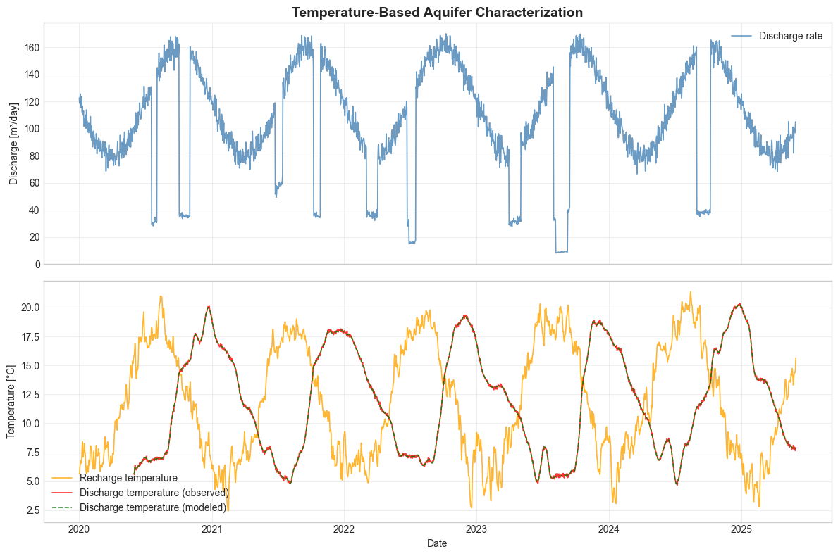
3. Model Validation and Visualization#
We compare observed and modeled temperature breakthrough curves to assess model performance.
[7]:
fig, (ax1, ax2) = plt.subplots(figsize=(12, 8), nrows=2, ncols=1, sharex=True)

# Flow rate subplot - convert to step format
xstep_flow, ystep_flow = step_plot_coords(tedges, df.flow)
ax1.set_title("Temperature-Based Aquifer Characterization", fontsize=14, fontweight="bold")
ax1.plot(xstep_flow, ystep_flow, label="Discharge rate", color="steelblue", alpha=0.8, linewidth=1.2)
ax1.set_ylabel("Discharge [m³/day]")
ax1.legend()
ax1.grid(True, alpha=0.3)

# Temperature subplot - convert all series to step format
xstep_temp, ystep_infiltration = step_plot_coords(tedges, df.cin)
_, ystep_extraction = step_plot_coords(tedges, df.cout)
_, ystep_modeled = step_plot_coords(tedges, df.cout_modeled)

ax2.plot(xstep_temp, ystep_infiltration, label="Recharge temperature", color="orange", alpha=0.8, linewidth=1.2)
ax2.plot(xstep_temp, ystep_extraction, label="Discharge temperature (observed)", color="red", alpha=0.8, linewidth=1.2)
ax2.plot(
    xstep_temp,
    ystep_modeled,
    label="Discharge temperature (modeled)",
    color="green",
    alpha=0.8,
    linewidth=1.2,
    linestyle="--",
)

ax2.set_xlabel("Date")
ax2.set_ylabel("Temperature [°C]")
ax2.legend()
ax2.grid(True, alpha=0.3)

plt.tight_layout()
plt.show()
4. Pore Volume Distribution Analysis#
We visualize the fitted gamma distribution representing spatial heterogeneity in pore volume. Each bin represents a different flow path through the aquifer.
[8]:
# Discretize gamma distribution into flow path bins
n_bins = 10  # Reduced for visualization clarity
alpha, beta = gamma_utils.mean_std_loc_to_alpha_beta(mean=mean, std=std)
gbins = gamma_utils.bins(alpha=alpha, beta=beta, n_bins=n_bins)

print(f"Gamma Distribution Parameters: alpha={alpha:.1f}, beta={beta:.1f}")
print(f"Discretized into {n_bins} equiprobable bins:")
print("-" * 80)
print(f"{'Bin':3s} {'Lower [m³]':10s} {'Upper [m³]':10s} {'E[V|bin]':10s} {'P(bin)':10s}")
print("-" * 80)

for i in range(n_bins):
    upper = f"{gbins['upper_bound'][i]:.1f}" if not np.isinf(gbins["upper_bound"][i]) else "∞"
    lower = f"{gbins['lower_bound'][i]:.1f}"
    expected = f"{gbins['expected_values'][i]:.1f}"
    prob = f"{gbins['probability_mass'][i]:.3f}"
    print(f"{i:3d} {lower:10s} {upper:10s} {expected:10s} {prob:10s}")
Gamma Distribution Parameters: alpha=419.4, beta=19.1
Discretized into 10 equiprobable bins:
--------------------------------------------------------------------------------
Bin Lower [m³] Upper [m³] E[V|bin]   P(bin)
--------------------------------------------------------------------------------
  0 0.0        7503.4     7328.6     0.100
  1 7503.4     7669.2     7592.5     0.100
  2 7669.2     7790.4     7731.9     0.100
  3 7790.4     7894.8     7843.4     0.100
  4 7894.8     7993.4     7944.3     0.100
  5 7993.4     8092.7     8042.7     0.100
  6 8092.7     8199.8     8145.2     0.100
  7 8199.8     8326.5     8260.8     0.100
  8 8326.5     8504.2     8408.3     0.100
  9 8504.2     ∞          8699.4     0.100
[9]:
# Plot the gamma distribution and bins
x = np.linspace(0, 1.1 * gbins["expected_values"][-1], 1000)
y = gamma_dist.pdf(x, alpha, scale=beta)

fig, ax = plt.subplots(figsize=(12, 8))
ax.set_title(
    f"Fitted Pore Volume Distribution\n(alpha={alpha:.1f}, beta={beta:.1f}, mean={mean:.0f} m³, std={std:.0f} m³)",
    fontsize=14,
    fontweight="bold",
)

ax.plot(x, y, label="Probability density function", color="navy", alpha=0.8, linewidth=2.5)
pdf_at_lower_bound = gamma_dist.pdf(gbins["lower_bound"], alpha, scale=beta)
ax.vlines(
    gbins["lower_bound"],
    0,
    pdf_at_lower_bound,
    color="red",
    alpha=0.6,
    linewidth=1.5,
    label="Bin boundaries",
)

ax.set_xlabel("Pore Volume [m³]")
ax.set_ylabel("Probability Density [m^-3]")
ax.legend()
ax.grid(True, alpha=0.3)

plt.tight_layout()
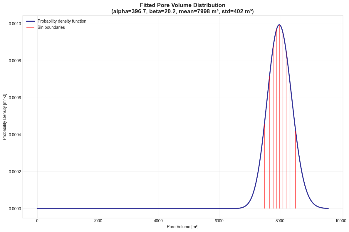
Results & Discussion#
The inverse modeling successfully recovered the aquifer pore volume distribution parameters. The fitted gamma distribution captures the heterogeneity in flow paths through the aquifer.
Practical Applications#
Contaminant Transport: Use fitted parameters to predict pollutant breakthrough
Well Field Design: Optimize extraction rates based on residence time requirements
Vulnerability Assessment: Identify fast flow paths that may compromise water quality
Key Takeaways#
Temperature as Natural Tracer: Temperature provides valuable information about aquifer properties without artificial injection
Inverse Modeling: Optimization techniques can extract quantitative aquifer parameters from field observations
Gamma Distribution: Effective model for representing aquifer heterogeneity in engineering applications
Thermal Retardation: Must account for heat exchange when using temperature data
Spin-up Period: Use :func:
~gwtransport.residence_time.fraction_explained_gammato determine when the model output is fully informed by the input signal