Note

This notebook is located in the ./examples directory of the gwtransport repository.

Residence Time Distribution Analysis#

Learning Objectives#

Calculate residence time distributions from aquifer pore volume distributions
Understand the difference between infiltration to extraction and extraction to infiltration residence time perspectives
Analyze temporal variations in groundwater residence times
Apply residence time concepts to contaminant transport and water quality assessment

Overview#

This notebook demonstrates how to calculate residence time distributions from aquifer pore volume distributions and flow rates. Residence time quantifies how long water spends in the aquifer, which is crucial for understanding contaminant transport and water quality.

Two Perspectives#

Infiltration to Extraction: How long until infiltrating water is extracted?
Extraction to Infiltration: How long ago was extracted water infiltrated?

Key Assumptions#

Stationary pore volume distribution (steady streamlines)
Known aquifer heterogeneity (from Example 1)

Background Reading#

Residence Time — Time in aquifer between infiltration and extraction
Pore Volume Distribution — Aquifer heterogeneity modeling
Retardation Factor — Slower movement due to sorption

Theoretical Background#

Residence Time#

Residence time represents the travel time of water through the aquifer:

\[t_{residence} = \frac{V_{pore}}{Q} \cdot R_f\]

where \(V_{pore}\) is pore volume [m³], \(Q\) is flow rate [m³/day], and \(R_f\) is the retardation factor [-].

Residence times vary over time due to seasonal flow rate changes and extraction rate variations. See residence time and retardation factor for background.

[1]:

import warnings

import matplotlib.pyplot as plt
import numpy as np

from gwtransport import gamma as gamma_utils
from gwtransport.examples import generate_temperature_example_data
from gwtransport.residence_time import fraction_explained, residence_time
from gwtransport.utils import step_plot_coords

# Set random seed for reproducibility
np.random.seed(42)
plt.style.use("seaborn-v0_8-whitegrid")

print("Libraries imported successfully")

Libraries imported successfully

1. Data Setup and Aquifer Parameters#

We use aquifer parameters typically obtained from Example 1 (temperature-based characterization) and generate flow data for residence time analysis.

[2]:

df, tedges = generate_temperature_example_data(
    date_start="2020-01-01",
    date_end="2025-05-31",
    flow_mean=120.0,  # Base flow rate [m³/day]
    flow_amplitude=40.0,  # Seasonal flow variation [m³/day]
    flow_noise=5.0,  # Random daily fluctuations [m³/day]
    cin_method="soil_temperature",  # Use real soil temperature data
    aquifer_pore_volume_gamma_mean=8000.0,  # True mean pore volume [m³]
    aquifer_pore_volume_gamma_std=400.0,  # True standard deviation [m³]
)

print("Dataset Summary:")
print(f"Period: {df.index[0].date()} to {df.index[-1].date()}")
print(f"Mean flow: {df['flow'].mean():.1f} m³/day")
print(f"Flow range: {df['flow'].min():.1f} - {df['flow'].max():.1f} m³/day")
print(
    f"Aquifer parameters: {df.attrs['aquifer_pore_volume_gamma_mean']:.0f} ± {df.attrs['aquifer_pore_volume_gamma_std']:.0f} m³"
)

print("Dataset Summary:")
print(f"Period: {df.index[0].date()} to {df.index[-1].date()}")
print(f"Mean flow: {df['flow'].mean():.1f} m³/day")
print(f"Mean infiltration temperature: {df['cin'].mean():.1f} °C")
print(f"Mean extraction temperature: {df['cout'].mean():.1f} °C")
print(f"True mean pore volume: {df.attrs['aquifer_pore_volume_gamma_mean']:.1f} m³")
print(f"True std deviation: {df.attrs['aquifer_pore_volume_gamma_std']:.1f} m³")

Dataset Summary:
Period: 2020-01-01 to 2025-05-31
Mean flow: 102.0 m³/day
Flow range: 4.5 - 169.7 m³/day
Aquifer parameters: 8000 ± 400 m³
Dataset Summary:
Period: 2020-01-01 to 2025-05-31
Mean flow: 102.0 m³/day
Mean infiltration temperature: 11.8 °C
Mean extraction temperature: 12.8 °C
True mean pore volume: 8000.0 m³
True std deviation: 400.0 m³

[3]:

# Discretize pore volume distribution for residence time calculation
n_bins = 1000  # High resolution for accurate calculations
bins = gamma_utils.bins(
    mean=df.attrs["aquifer_pore_volume_gamma_mean"], std=df.attrs["aquifer_pore_volume_gamma_std"], n_bins=n_bins
)

print(f"Pore volume distribution discretized into {n_bins} bins")
print(f"Bin range: {bins['expected_values'].min():.0f} - {bins['expected_values'].max():.0f} m³")
print(
    f"Mean residence time (no retardation): {df.attrs['aquifer_pore_volume_gamma_mean'] / df['flow'].mean():.1f} days"
)
print(
    f"Mean residence time (with retardation): {df.attrs['aquifer_pore_volume_gamma_mean'] / df['flow'].mean() * df.attrs['retardation_factor']:.1f} days"
)

Pore volume distribution discretized into 1000 bins
Bin range: 6722 - 9417 m³
Mean residence time (no retardation): 78.4 days
Mean residence time (with retardation): 156.8 days

2. Infiltration to Extraction Residence Time Analysis#

Calculate how long infiltrating water takes to be extracted. We compute residence times for both water flow (conservative tracer) and thermal transport (with retardation).

[4]:

print("Computing infiltration to extraction residence times...")

# Water residence time (no retardation)
rt_infiltration_to_extraction_water = residence_time(
    flow=df.flow,
    flow_tedges=tedges,
    aquifer_pore_volumes=bins["expected_values"],
    retardation_factor=1.0,  # Conservative tracer (water flow)
    direction="infiltration_to_extraction",
)

# Thermal residence time (with retardation)
rt_infiltration_to_extraction_thermal = residence_time(
    flow=df.flow,
    flow_tedges=tedges,
    aquifer_pore_volumes=bins["expected_values"],
    retardation_factor=df.attrs["retardation_factor"],  # Heat transport (slower)
    direction="infiltration_to_extraction",
)

print(f"Infiltration to extraction residence time arrays shape: {rt_infiltration_to_extraction_water.shape}")
print(
    f"({rt_infiltration_to_extraction_water.shape[0]} flow paths x {rt_infiltration_to_extraction_water.shape[1]} time steps)"
)

Computing infiltration to extraction residence times...
Infiltration to extraction residence time arrays shape: (1000, 1978)
(1000 flow paths x 1978 time steps)

[5]:

# Statistical analysis of residence time distributions
quantiles = [1, 10, 90, 99]  # Percentiles for uncertainty bounds
quantile_headers = [f"rt_infiltration_to_extraction_water_{q}%" for q in quantiles]

with warnings.catch_warnings():
    warnings.filterwarnings(action="ignore", message="Mean of empty slice")
    warnings.filterwarnings(action="ignore", message="All-NaN slice encountered")

    # Calculate mean residence times
    df["rt_infiltration_to_extraction_water_mean"] = np.nanmean(rt_infiltration_to_extraction_water, axis=0)
    df["rt_infiltration_to_extraction_thermal_mean"] = np.nanmean(rt_infiltration_to_extraction_thermal, axis=0)

    # Calculate percentiles for uncertainty analysis
    df[quantile_headers] = np.nanpercentile(rt_infiltration_to_extraction_water, quantiles, axis=0).T

print("Infiltration to extraction residence time statistics calculated")
print(f"Mean water residence time: {df['rt_infiltration_to_extraction_water_mean'].mean():.1f} days")
print(f"Mean thermal residence time: {df['rt_infiltration_to_extraction_thermal_mean'].mean():.1f} days")
print(
    f"Retardation effect: {df['rt_infiltration_to_extraction_thermal_mean'].mean() / df['rt_infiltration_to_extraction_water_mean'].mean():.1f}x"
)
print(
    f"({rt_infiltration_to_extraction_water.shape[0]} flow paths x {rt_infiltration_to_extraction_water.shape[1]} time steps)"
)

Infiltration to extraction residence time statistics calculated
Mean water residence time: 82.9 days
Mean thermal residence time: 156.1 days
Retardation effect: 1.9x
(1000 flow paths x 1978 time steps)

Fraction Explained: Assessing Spin-Up#

During the initial period, some flow paths do not yet have sufficient flow history to compute a valid residence time (the residence time is NaN). The :func:~gwtransport.residence_time.fraction_explained function quantifies which fraction of pore volumes have valid residence times at each time step. A value of 1.0 means all flow paths are fully informed.

[6]:

# Compute fraction of pore volumes with valid residence times
frac_explained_forward = fraction_explained(rt=rt_infiltration_to_extraction_water)

# Find the first date where all flow paths are fully informed
fully_explained_mask = frac_explained_forward >= 1.0
if fully_explained_mask.any():
    first_fully_explained = df.index[fully_explained_mask][0]
    print(f"Spin-up period ends: {first_fully_explained.date()}")
else:
    print("Warning: Not all pore volumes are fully explained within the data period")

print(f"Fraction explained at start: {frac_explained_forward[0]:.2f}")
print(f"Fraction explained at end: {frac_explained_forward[-1]:.2f}")

Spin-up period ends: 2020-01-01
Fraction explained at start: 1.00
Fraction explained at end: 0.00

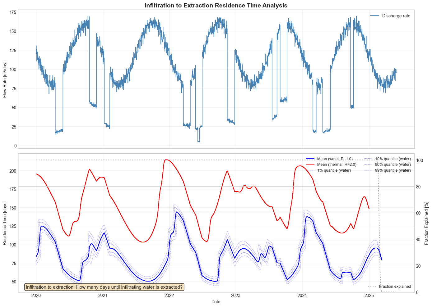
3. Infiltration to Extraction Residence Time Visualization#

Visualize how residence times vary over time and compare water vs. thermal transport.

[7]:

fig, ax = plt.subplots(2, 1, figsize=(14, 10), sharex=True)

# Flow rate subplot - convert to step format
xstep_flow, ystep_flow = step_plot_coords(tedges, df.flow)
ax[0].plot(xstep_flow, ystep_flow, label="Discharge rate", color="steelblue", linewidth=1.2)
ax[0].set_ylabel("Flow Rate [m³/day]")
ax[0].set_title("Infiltration to Extraction Residence Time Analysis", fontsize=14, fontweight="bold")
ax[0].legend(loc="upper right")
ax[0].grid(True, alpha=0.3)

# Residence time subplot - convert all series to step format
xstep_rt, ystep_rt_water = step_plot_coords(tedges, df.rt_infiltration_to_extraction_water_mean)
_, ystep_rt_thermal = step_plot_coords(tedges, df.rt_infiltration_to_extraction_thermal_mean)

ax[1].plot(
    xstep_rt,
    ystep_rt_water,
    label="Mean (water, R=1.0)",
    color="blue",
    linewidth=1.5,
)
ax[1].plot(
    xstep_rt,
    ystep_rt_thermal,
    label=f"Mean (thermal, R={df.attrs['retardation_factor']:.1f})",
    color="red",
    linewidth=1.5,
)

# Add uncertainty bounds
for q in quantiles:
    alpha_val = 0.4 if q in {10, 90} else 0.3
    linestyle = "--" if q in {1, 99} else "-."
    _, ystep_quantile = step_plot_coords(tedges, df[f"rt_infiltration_to_extraction_water_{q}%"])
    ax[1].plot(
        xstep_rt,
        ystep_quantile,
        label=f"{q}% quantile (water)",
        color="blue",
        alpha=alpha_val,
        linewidth=0.8,
        linestyle=linestyle,
    )

ax[1].set_ylabel("Residence Time [days]")
ax[1].set_xlabel("Date")
ax[1].legend(loc="upper right", ncol=2, fontsize=9)
ax[1].grid(True, alpha=0.3)

# Add fraction explained on twin axis
ax1b = ax[1].twinx()
ax1b.plot(
    *step_plot_coords(tedges, frac_explained_forward * 100),
    color="gray",
    linewidth=1.5,
    linestyle=":",
    alpha=0.8,
    label="Fraction explained",
)
ax1b.set_ylabel("Fraction Explained [%]")
ax1b.set_ylim(0, 105)
ax1b.legend(loc="lower right", fontsize=9)

# Add explanatory text
ax[1].text(
    0.02,
    0.02,
    "Infiltration to extraction: How many days until infiltrating water is extracted?",
    ha="left",
    va="bottom",
    transform=ax[1].transAxes,
    fontsize=11,
    bbox={"boxstyle": "round,pad=0.3", "facecolor": "wheat", "alpha": 0.8},
)

plt.tight_layout()

plt.show()

../_images/examples_02_Residence_Time_Analysis_13_0.png

4. Extraction to Infiltration Residence Time Analysis#

Calculate when currently extracted water was originally infiltrated. This perspective is crucial for source identification and age dating.

[8]:

print("Computing extraction to infiltration residence times...")

# Water residence time (no retardation)
rt_extraction_to_infiltration_water = residence_time(
    flow=df.flow,
    flow_tedges=tedges,
    aquifer_pore_volumes=bins["expected_values"],
    retardation_factor=1.0,
    direction="extraction_to_infiltration",
)

# Thermal residence time (with retardation)
rt_extraction_to_infiltration_thermal = residence_time(
    flow=df.flow,
    flow_tedges=tedges,
    aquifer_pore_volumes=bins["expected_values"],
    retardation_factor=df.attrs["retardation_factor"],
    direction="extraction_to_infiltration",
)

print(f"Extraction to infiltration residence time arrays shape: {rt_extraction_to_infiltration_water.shape}")

Computing extraction to infiltration residence times...
Extraction to infiltration residence time arrays shape: (1000, 1978)

[9]:

# Statistical analysis for extraction to infiltration residence times
quantile_headers_extraction_to_infiltration = [f"rt_extraction_to_infiltration_water_{q}%" for q in quantiles]

with warnings.catch_warnings():
    warnings.filterwarnings(action="ignore", message="Mean of empty slice")
    warnings.filterwarnings(action="ignore", message="All-NaN slice encountered")

    # Calculate mean residence times
    df["rt_extraction_to_infiltration_water_mean"] = np.nanmean(rt_extraction_to_infiltration_water, axis=0)
    df["rt_extraction_to_infiltration_thermal_mean"] = np.nanmean(rt_extraction_to_infiltration_thermal, axis=0)

    # Calculate percentiles
    df[quantile_headers_extraction_to_infiltration] = np.nanpercentile(
        rt_extraction_to_infiltration_water, quantiles, axis=0
    ).T

# Compute fraction explained for extraction to infiltration direction
frac_explained_backward = fraction_explained(rt=rt_extraction_to_infiltration_water)

print("Extraction to infiltration residence time statistics calculated")
print(
    f"Mean extraction to infiltration water residence time: {df['rt_extraction_to_infiltration_water_mean'].mean():.1f} days"
)
print(
    f"Mean extraction to infiltration thermal residence time: {df['rt_extraction_to_infiltration_thermal_mean'].mean():.1f} days"
)

fully_explained_backward_mask = frac_explained_backward >= 1.0
if fully_explained_backward_mask.any():
    print(f"Spin-up period ends: {df.index[fully_explained_backward_mask][0].date()}")

Extraction to infiltration residence time statistics calculated
Mean extraction to infiltration water residence time: 82.8 days
Mean extraction to infiltration thermal residence time: 156.0 days
Spin-up period ends: 2020-04-10

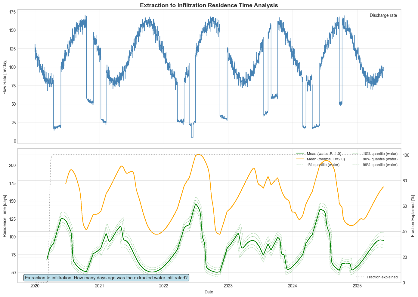
5. Extraction to Infiltration Residence Time Visualization#

Show how the age of extracted water varies over time, revealing the temporal dynamics of groundwater flow.

[10]:

fig, ax = plt.subplots(2, 1, figsize=(14, 10), sharex=True)

# Flow rate subplot - convert to step format
xstep_flow, ystep_flow = step_plot_coords(tedges, df.flow)
ax[0].plot(xstep_flow, ystep_flow, label="Discharge rate", color="steelblue", linewidth=1.2)
ax[0].set_ylabel("Flow Rate [m³/day]")
ax[0].set_title("Extraction to Infiltration Residence Time Analysis", fontsize=14, fontweight="bold")
ax[0].legend(loc="upper right")
ax[0].grid(True, alpha=0.3)

# Residence time subplot - convert all series to step format
xstep_rt, ystep_rt_water = step_plot_coords(tedges, df.rt_extraction_to_infiltration_water_mean)
_, ystep_rt_thermal = step_plot_coords(tedges, df.rt_extraction_to_infiltration_thermal_mean)

ax[1].plot(
    xstep_rt,
    ystep_rt_water,
    label="Mean (water, R=1.0)",
    color="green",
    linewidth=1.5,
)
ax[1].plot(
    xstep_rt,
    ystep_rt_thermal,
    label=f"Mean (thermal, R={df.attrs['retardation_factor']:.1f})",
    color="orange",
    linewidth=1.5,
)

# Add uncertainty bounds for water
for q in quantiles:
    alpha_val = 0.4 if q in {10, 90} else 0.3
    linestyle = "--" if q in {1, 99} else "-."
    _, ystep_quantile = step_plot_coords(tedges, df[f"rt_extraction_to_infiltration_water_{q}%"])
    ax[1].plot(
        xstep_rt,
        ystep_quantile,
        label=f"{q}% quantile (water)",
        color="green",
        alpha=alpha_val,
        linewidth=0.8,
        linestyle=linestyle,
    )

ax[1].set_ylabel("Residence Time [days]")
ax[1].set_xlabel("Date")
ax[1].legend(loc="upper right", ncol=2, fontsize=9)
ax[1].grid(True, alpha=0.3)

# Add fraction explained on twin axis
ax1b = ax[1].twinx()
ax1b.plot(
    *step_plot_coords(tedges, frac_explained_backward * 100),
    color="gray",
    linewidth=1.5,
    linestyle=":",
    alpha=0.8,
    label="Fraction explained",
)
ax1b.set_ylabel("Fraction Explained [%]")
ax1b.set_ylim(0, 105)
ax1b.legend(loc="lower right", fontsize=9)

# Add explanatory text
ax[1].text(
    0.02,
    0.02,
    "Extraction to infiltration: How many days ago was the extracted water infiltrated?",
    ha="left",
    va="bottom",
    transform=ax[1].transAxes,
    fontsize=11,
    bbox={"boxstyle": "round,pad=0.3", "facecolor": "lightblue", "alpha": 0.8},
)

plt.tight_layout()

plt.show()

../_images/examples_02_Residence_Time_Analysis_18_0.png

Results & Discussion#

Flow Rate Dependencies#

Residence times show strong inverse correlation with flow rates — higher flows yield shorter residence times. Both infiltration-to-extraction and extraction-to-infiltration perspectives yield comparable averages but differ in temporal patterns.

Retardation Effects#

Thermal retardation factor of 2.0 effectively doubles residence times, which must be considered in heat transport applications.

Practical Applications#

Infiltration to extraction: Use for contaminant arrival time predictions and spill response planning
Extraction to infiltration: Use for source identification and age dating
Seasonal variations: Consider flow variations when designing monitoring and management strategies

Key Takeaways#

Two Perspectives: Infiltration-to-extraction and extraction-to-infiltration residence times answer different but complementary questions
Flow Rate Control: Higher flows lead to shorter residence times and faster transport
Retardation Effects: Must account for tracer-specific retardation in transport analysis
Spin-up Assessment: Use :func:~gwtransport.residence_time.fraction_explained to identify when model output is fully informed by input signal

Residence Time Distribution Analysis

Contents

Residence Time Distribution Analysis#

Learning Objectives#

Overview#

Two Perspectives#

Key Assumptions#

Background Reading#

Theoretical Background#

Residence Time#

1. Data Setup and Aquifer Parameters#

2. Infiltration to Extraction Residence Time Analysis#

Fraction Explained: Assessing Spin-Up#

3. Infiltration to Extraction Residence Time Visualization#

4. Extraction to Infiltration Residence Time Analysis#

5. Extraction to Infiltration Residence Time Visualization#

Results & Discussion#

Flow Rate Dependencies#

Retardation Effects#

Practical Applications#

Key Takeaways#