Note

This notebook is located in the ./examples directory of the gwtransport repository.

Pathogen Removal in Bank Filtration Systems#

Learning Objectives#

Understand log-removal concepts for pathogen treatment assessment
Calculate pathogen removal efficiency in groundwater treatment systems
Learn how heterogeneous systems affect overall performance
Apply residence time analysis to water treatment design
Analyze seasonal variations in treatment performance

Overview#

This notebook demonstrates how to calculate pathogen removal efficiency in groundwater treatment systems using log-removal analysis. Understanding pathogen removal is crucial for safe drinking water production from riverbank filtration and managed aquifer recharge systems.

Real-World Context#

Bank filtration is widely used in Europe for drinking water treatment. River water infiltrates through riverbank sediments, where pathogens are naturally filtered out through physical straining and biological decay. The longer water stays underground, the more pathogens are removed.

Applications#

Drinking water treatment design
Bank filtration system optimization
Risk assessment for water supplies
Treatment performance evaluation
Treatment performance monitoring

Key Concepts#

Log-removal: Logarithmic scale for pathogen reduction
Residence time dependency: Longer contact time = better removal
Heterogeneous systems: Multiple flow paths with different performance
Treatment efficiency: Quantifying pathogen removal performance

Background Reading#

Residence Time - Contact time determines removal efficiency
Pore Volume Distribution - Flow path heterogeneity affects overall performance
No Reactions Assumption - When first-order decay applies

Theoretical Background#

Log-Removal Fundamentals#

Log-removal quantifies pathogen reduction on a logarithmic scale:

\[\text{Log-removal} = \log_{10}\left(\frac{C_{in}}{C_{out}}\right)\]

Where:

\(C_{in}\): Input pathogen concentration
\(C_{out}\): Output pathogen concentration

Practical Interpretation:

1 log10 = 90% removal (1 in 10 pathogens remain)
2 log10 = 99% removal (1 in 100 pathogens remain)
3 log10 = 99.9% removal (1 in 1000 pathogens remain)

Pathogen Removal Mechanisms#

During soil passage, pathogen removal consists of two distinct mechanisms (Schijven and Hassanizadeh, 2000):

Inactivation (time-dependent): Pathogens lose infectivity over time through biological decay. This follows first-order kinetics:

\[\text{LR}_\text{decay} = \mu \cdot t_{residence}\]

where \(\mu\) is the log10 decay rate [log10/day]. The inactivation rate depends strongly on temperature and pathogen type.
Attachment (geometry-dependent): Pathogens are physically removed by adsorption to soil grains and straining. This depends on aquifer geometry, travel distance, soil properties, and pH. At the Castricum dune recharge site, Schijven et al. (1999) found that attachment contributed approximately 97% of total MS2 removal.

Total log-removal = LR_decay (time-dependent, modeled by gwtransport) + LR_attachment (geometry-dependent, user-specified)

The gwtransport.logremoval module models only the time-dependent decay component. Users add the geometry-dependent attachment component based on site-specific knowledge.

Connection to Radioactive Decay#

The first-order decay model is mathematically identical to radioactive decay used in tracer dating. The natural-log decay rate constant \(\lambda\) [1/day] is related to \(\mu\) by:

\[\lambda = \mu \cdot \ln(10) \quad \Leftrightarrow \quad \mu = \frac{\lambda}{\ln(10)}\]

Published decay rates from tracer studies can be converted using decay_rate_to_log10_decay_rate().

Heterogeneous Systems#

For systems with multiple flow paths, the overall log-removal is weighted toward lower values (shorter residence times), providing natural safety margins in design.

[1]:

from pathlib import Path

import matplotlib.pyplot as plt
import numpy as np

from gwtransport import gamma as gamma_utils
from gwtransport.examples import generate_example_data
from gwtransport.logremoval import (
    decay_rate_to_log10_decay_rate,
    gamma_find_flow_for_target_mean,
    gamma_mean,
    parallel_mean,
    residence_time_to_log_removal,
)
from gwtransport.residence_time import residence_time

# Set random seed for reproducibility
np.random.seed(42)
plt.style.use("seaborn-v0_8-whitegrid")

print("Libraries imported successfully")

Libraries imported successfully

1. Understanding Pathogen Inactivation Rates#

Pathogen inactivation rates vary significantly between virus types and temperatures. Schijven and Hassanizadeh (2000) compiled inactivation rates from multiple studies and found that the temperature dependence follows: ln(mu_l) = a*T + b, where T is the groundwater temperature in degrees Celsius.

The table below shows inactivation rates at 10 degrees C for common model viruses:

[2]:

print("=== Pathogen Inactivation Rates ===")
print("From Schijven and Hassanizadeh (2000), Table 7")
print("Temperature regression: ln(mu_l) = a*T + b\n")

# Inactivation rate regression parameters from Schijven & Hassanizadeh (2000) Table 7
# mu_l is the natural-log inactivation rate [day^-1]
# ln(mu_l) = a * T + b, where T is temperature in degrees C
pathogen_params = {
    "MS2": {"a": 0.12, "b": -3.5, "R2": 0.85},
    "PRD1": {"a": 0.09, "b": -4.0, "R2": 0.71},
    "Poliovirus 1": {"a": 0.033, "b": -2.4, "R2": 0.07},
    "Echovirus 1": {"a": 0.12, "b": -3.0, "R2": 0.71},
    "HAV": {"a": -0.024, "b": -1.4, "R2": 0.08},
}


def inactivation_rate_log10(temperature, a, b):
    """Compute log10 inactivation rate [log10/day] at temperature [deg C]."""
    mu_l = np.exp(a * temperature + b)  # natural-log rate [1/day]
    return mu_l / np.log(10)  # convert to log10 rate [log10/day]


# Evaluate at T = 10 deg C (typical Dutch groundwater)
T_ref = 10.0
print(f"Inactivation rates at T = {T_ref:.0f} deg C:")
print(f"{'Virus':<16} {'mu_l [1/day]':>12} {'mu [log10/day]':>15} {'Temp. sensitivity':>18}")
print("-" * 65)

log10_decay_rates = {}
for virus, params in pathogen_params.items():
    mu_l = np.exp(params["a"] * T_ref + params["b"])
    mu_log10 = mu_l / np.log(10)
    log10_decay_rates[virus] = mu_log10
    r2_str = f"R2={params['R2']:.0%}" if params["R2"] > 0.5 else f"R2={params['R2']:.0%} (weak)"
    print(f"  {virus:<14} {mu_l:>12.4f} {mu_log10:>15.4f} {r2_str:>18}")

print("\nNote: These are INACTIVATION rates only (time-dependent decay).")
print("Total pathogen removal also includes attachment (geometry-dependent),")
print("which typically dominates and is not modeled by gwtransport.")

=== Pathogen Inactivation Rates ===
From Schijven and Hassanizadeh (2000), Table 7
Temperature regression: ln(mu_l) = a*T + b

Inactivation rates at T = 10 deg C:
Virus            mu_l [1/day]  mu [log10/day]  Temp. sensitivity
-----------------------------------------------------------------
  MS2                  0.1003          0.0435             R2=85%
  PRD1                 0.0450          0.0196             R2=71%
  Poliovirus 1         0.1262          0.0548       R2=7% (weak)
  Echovirus 1          0.1653          0.0718             R2=71%
  HAV                  0.1940          0.0842       R2=8% (weak)

Note: These are INACTIVATION rates only (time-dependent decay).
Total pathogen removal also includes attachment (geometry-dependent),
which typically dominates and is not modeled by gwtransport.

[3]:

print("=== Converting Published Decay Rates ===")
print("Example: MS2 inactivation rate from Schijven et al. (1999) Castricum field study\n")

# MS2 free virus inactivation rate at 5 deg C from Castricum field study
# Published as natural-log rate: mu_f = 0.03 day^-1
published_decay_rate = 0.03  # 1/day (natural-log inactivation rate for MS2 at 5 deg C)

# Convert to log10 decay rate
converted_rate = decay_rate_to_log10_decay_rate(published_decay_rate)

print(f"Published natural-log inactivation rate (lambda): {published_decay_rate} 1/day")
print(f"Converted log10 decay rate (mu): {converted_rate:.4f} log10/day")
print(f"\nVerification: mu * ln(10) = {converted_rate * np.log(10):.4f} (should equal lambda)")

# Compare with regression estimate
t_ref = 5.0
regression_rate = inactivation_rate_log10(t_ref, **{k: v for k, v in pathogen_params["MS2"].items() if k != "R2"})
print(f"\nRegression estimate for MS2 at {t_ref:.0f} deg C: {regression_rate:.4f} log10/day")
print(f"Field measurement at {t_ref:.0f} deg C: {converted_rate:.4f} log10/day")

# Show what this means for a typical residence time
mean_residence_time = 76.0  # days (example from article)
print(f"\nFor a mean residence time of {mean_residence_time:.0f} days:")
print(
    f"  LR_decay (inactivation only) = {converted_rate:.4f} * {mean_residence_time:.0f} = {converted_rate * mean_residence_time:.2f} log10"
)
print("  This is just the time-dependent component.")
print("  The user must add site-specific attachment removal separately.")

=== Converting Published Decay Rates ===
Example: MS2 inactivation rate from Schijven et al. (1999) Castricum field study

Published natural-log inactivation rate (lambda): 0.03 1/day
Converted log10 decay rate (mu): 0.0130 log10/day

Verification: mu * ln(10) = 0.0300 (should equal lambda)

Regression estimate for MS2 at 5 deg C: 0.0239 log10/day
Field measurement at 5 deg C: 0.0130 log10/day

For a mean residence time of 76 days:
  LR_decay (inactivation only) = 0.0130 * 76 = 0.99 log10
  This is just the time-dependent component.
  The user must add site-specific attachment removal separately.

2. Heterogeneous System Performance#

Bank filtration systems have multiple flow paths with different residence times. The overall log-removal is weighted toward lower values (shorter residence times).

[4]:

print("=== Heterogeneous System Analysis ===")
print("Multiple flow paths with different residence times\n")

# Three flow paths with different log-removal efficiencies
unit_removals = np.array([0.5, 1.0, 1.5])  # log10 values for each path

# Correct method: parallel_mean() accounts for flow-weighted averaging
combined_removal = parallel_mean(log_removals=unit_removals)

print("Flow Path Performance:")
for i, removal in enumerate(unit_removals):
    efficiency = (1 - 10 ** (-removal)) * 100
    print(f"  Path {i + 1}: {removal:.1f} log10 -> {efficiency:.1f}% removal")

print("\nOverall System Performance:")
combined_efficiency = (1 - 10 ** (-combined_removal)) * 100
print(f"  Combined log-removal: {combined_removal:.2f} log10 -> {combined_efficiency:.1f}% removal")

print("\nNote: Overall performance is weighted toward the worst-performing paths")
print("(shortest residence times), ensuring conservative design.")

=== Heterogeneous System Analysis ===
Multiple flow paths with different residence times

Flow Path Performance:
  Path 1: 0.5 log10 -> 68.4% removal
  Path 2: 1.0 log10 -> 90.0% removal
  Path 3: 1.5 log10 -> 96.8% removal

Overall System Performance:
  Combined log-removal: 0.83 log10 -> 85.1% removal

Note: Overall performance is weighted toward the worst-performing paths
(shortest residence times), ensuring conservative design.

3. Design Application - Achieving Target Removal Efficiency#

Water treatment facilities aim to achieve specific pathogen removal targets. We demonstrate how to design systems that achieve desired removal efficiency.

[5]:

print("=== Design Application ===")
print("Design challenge: Achieve target inactivation for safe drinking water\n")

# Define aquifer characteristics (small riverbank aquifer)
mean_pore_volume = 1000.0  # m3 (total water-filled space)
std_pore_volume = 300.0  # m3 (variability in pore volume)
flow_rate = 50.0  # m3/day (water extraction rate)

# Convert aquifer properties to gamma distribution parameters
alpha, beta = gamma_utils.mean_std_to_alpha_beta(mean=mean_pore_volume, std=std_pore_volume)

# Use MS2 at 10 deg C as the design pathogen (worst-case model virus)
log10_decay_rate = log10_decay_rates["MS2"]  # ~0.043 log10/day

# Target inactivation level (decay component only)
target_decay = 3.0  # log10 inactivation target
print(f"Pathogen: MS2 at 10 deg C (mu = {log10_decay_rate:.4f} log10/day)")
print(f"Target inactivation (decay only): {target_decay} log10")

# Calculate effective decay at current flow
rt_alpha = alpha
rt_beta = beta / flow_rate
mean_log_removal = gamma_mean(rt_alpha=rt_alpha, rt_beta=rt_beta, log10_decay_rate=log10_decay_rate)

mean_residence_time = mean_pore_volume / flow_rate
print(f"\nAt flow rate {flow_rate} m3/day (mean RT = {mean_residence_time:.0f} days):")
print(f"  Effective inactivation: {mean_log_removal:.2f} log10")

# Find the maximum flow rate that still achieves the inactivation target
required_flow = gamma_find_flow_for_target_mean(
    target_mean=target_decay,
    apv_alpha=alpha,
    apv_beta=beta,
    log10_decay_rate=log10_decay_rate,
)

required_residence_time = mean_pore_volume / required_flow

print(f"\nMaximum flow for {target_decay} log10 inactivation target:")
print(f"  Maximum flow rate: {required_flow:.1f} m3/day")
print(f"  Required mean residence time: {required_residence_time:.1f} days")

# Compare all pathogens
print(f"\nMaximum flow rates for {target_decay} log10 inactivation target (all pathogens):")
for virus, mu in log10_decay_rates.items():
    max_flow = gamma_find_flow_for_target_mean(
        target_mean=target_decay,
        apv_alpha=alpha,
        apv_beta=beta,
        log10_decay_rate=mu,
    )
    print(f"  {virus:<16}: {max_flow:>6.1f} m3/day (mu = {mu:.4f} log10/day)")

=== Design Application ===
Design challenge: Achieve target inactivation for safe drinking water

Pathogen: MS2 at 10 deg C (mu = 0.0435 log10/day)
Target inactivation (decay only): 3.0 log10

At flow rate 50.0 m3/day (mean RT = 20 days):
  Effective inactivation: 0.80 log10

Maximum flow for 3.0 log10 inactivation target:
  Maximum flow rate: 10.5 m3/day
  Required mean residence time: 95.5 days

Maximum flow rates for 3.0 log10 inactivation target (all pathogens):
  MS2             :   10.5 m3/day (mu = 0.0435 log10/day)
  PRD1            :    4.7 m3/day (mu = 0.0196 log10/day)
  Poliovirus 1    :   13.2 m3/day (mu = 0.0548 log10/day)
  Echovirus 1     :   17.3 m3/day (mu = 0.0718 log10/day)
  HAV             :   20.3 m3/day (mu = 0.0842 log10/day)

4. Real-World Scenario - Seasonal Variations#

In reality, river flows change seasonally, affecting bank filtration performance. We simulate a multi-year system to see how log-removal varies with changing conditions.

[6]:

print("=== Seasonal Flow Data Generation ===")

# Generate realistic flow data with seasonal patterns
df, tedges = generate_example_data(
    date_start="2020-01-01",
    date_end="2025-05-31",
    flow_mean=120.0,  # Base flow rate [m³/day]
    flow_amplitude=40.0,  # Seasonal flow variation [m³/day]
    flow_noise=5.0,  # Random daily fluctuations [m³/day]
    temp_infiltration_method="soil_temperature",  # Use real soil temperature data
    aquifer_pore_volume_gamma_mean=8000.0,  # True mean pore volume [m³]
    aquifer_pore_volume_gamma_std=400.0,  # True standard deviation [m³]
    retardation_factor=2.0,  # Thermal retardation factor [-]
)

# Set up aquifer characteristics for this larger system
bins = gamma_utils.bins(
    mean=df.attrs["aquifer_pore_volume_gamma_mean"], std=df.attrs["aquifer_pore_volume_gamma_std"], n_bins=1000
)  # High resolution

print(f"Dataset: {len(df)} days from {df.index[0].date()} to {df.index[-1].date()}")
print(f"Flow range: {df['flow'].min():.1f} - {df['flow'].max():.1f} m³/day")
print(
    f"Aquifer: {df.attrs['aquifer_pore_volume_gamma_mean']:.0f} ± {df.attrs['aquifer_pore_volume_gamma_std']:.0f} m³ pore volume"
)

=== Seasonal Flow Data Generation ===
Dataset: 1978 days from 2020-01-01 to 2025-05-31
Flow range: 8.1 - 170.0 m³/day
Aquifer: 8000 ± 400 m³ pore volume

[7]:

print("\nComputing inactivation for multiple pathogens over time...")

# Calculate residence time distribution for water flow
rt_infiltration_to_extraction_water = residence_time(
    flow=df.flow,
    flow_tedges=tedges,
    aquifer_pore_volumes=bins["expected_values"],
    retardation_factor=1.0,  # Water (conservative tracer)
    direction="infiltration_to_extraction",
)

# Compute log-removal for each pathogen
for virus, mu in log10_decay_rates.items():
    col = f"lr_decay_{virus}"
    log_removal_array = residence_time_to_log_removal(
        residence_times=rt_infiltration_to_extraction_water,
        log10_decay_rate=mu,
    )
    df[col] = parallel_mean(log_removals=log_removal_array, axis=0)

print("Time series calculation completed for all pathogens")
print("\nInactivation ranges (decay component only):")
for virus in log10_decay_rates:
    col = f"lr_decay_{virus}"
    print(f"  {virus:<16}: {df[col].min():.2f} - {df[col].max():.2f} log10")


Computing inactivation for multiple pathogens over time...
Time series calculation completed for all pathogens

Inactivation ranges (decay component only):
  MS2             : 2.16 - 4.84 log10
  PRD1            : 0.98 - 2.18 log10
  Poliovirus 1    : 2.72 - 6.08 log10
  Echovirus 1     : 3.55 - 7.94 log10
  HAV             : 4.16 - 9.30 log10

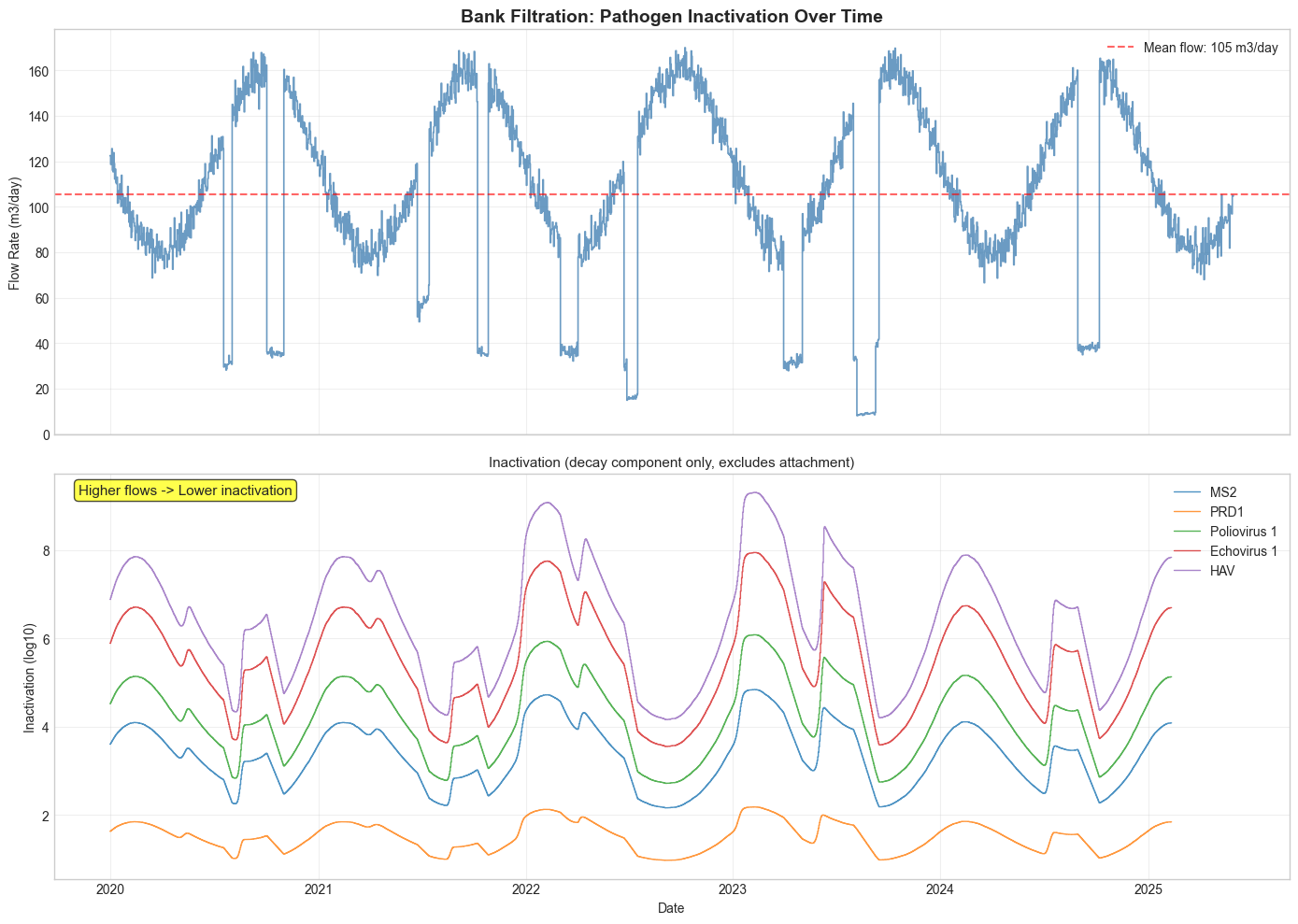
5. Performance Visualization#

[8]:

# Create time series plot showing inactivation for multiple pathogens
fig, (ax1, ax2) = plt.subplots(2, 1, figsize=(14, 10), sharex=True)

# Helper for step plots
xstep = np.repeat(tedges, 2)[1:-1]


def _step(values):
    """Repeat each value for step-plot visualization."""
    return np.repeat(values, 2)


# Plot 1: Flow rate over time
ax1.plot(xstep, _step(df.flow), color="steelblue", linewidth=1.2, alpha=0.8)
ax1.set_ylabel("Flow Rate (m3/day)")
ax1.set_title("Bank Filtration: Pathogen Inactivation Over Time", fontsize=14, fontweight="bold")
ax1.grid(True, alpha=0.3)
ax1.axhline(
    y=df.flow.mean(),
    color="red",
    linestyle="--",
    alpha=0.6,
    label=f"Mean flow: {df.flow.mean():.0f} m3/day",
)
ax1.legend()

# Plot 2: Inactivation for each pathogen
colors = {"MS2": "C0", "PRD1": "C1", "Poliovirus 1": "C2", "Echovirus 1": "C3", "HAV": "C4"}
for virus in log10_decay_rates:
    col = f"lr_decay_{virus}"
    ax2.plot(xstep, _step(df[col]), color=colors[virus], linewidth=1.0, alpha=0.8, label=virus)

ax2.set_ylabel("Inactivation (log10)")
ax2.set_xlabel("Date")
ax2.grid(True, alpha=0.3)
ax2.legend(loc="upper right")
ax2.set_title("Inactivation (decay component only, excludes attachment)", fontsize=11)

ax2.text(
    0.02,
    0.95,
    "Higher flows -> Lower inactivation",
    transform=ax2.transAxes,
    fontsize=11,
    bbox={"boxstyle": "round,pad=0.3", "facecolor": "yellow", "alpha": 0.7},
)

plt.tight_layout()
out_path = Path("03_log_removal_time_series.png")
plt.savefig(out_path, dpi=300, bbox_inches="tight")
plt.show()
print(f"Time series plot saved to: {out_path}")

../_images/examples_03_Pathogen_Removal_Bank_Filtration_15_0.png

Time series plot saved to: 03_log_removal_time_series.png

6. Performance Summary and Analysis#

[9]:

# Summary statistics for all pathogens
print("Performance Summary (inactivation component only):")
print("=" * 65)

for virus, mu in log10_decay_rates.items():
    col = f"lr_decay_{virus}"
    min_lr = df[col].min()
    max_lr = df[col].max()
    mean_lr = df[col].mean()
    std_lr = df[col].std()
    print(f"\n{virus} (mu = {mu:.4f} log10/day at 10 deg C):")
    print(f"  Range: {min_lr:.2f} - {max_lr:.2f} log10")
    print(f"  Mean:  {mean_lr:.2f} +/- {std_lr:.2f} log10")

print("\n" + "=" * 65)
print("\nRemember: Total pathogen removal = inactivation + attachment.")
print("The attachment component (geometry-dependent) must be added separately")
print("based on site-specific data. At the Castricum site (Schijven et al., 1999),")
print("attachment contributed ~97% of total MS2 removal.")

Performance Summary (inactivation component only):
=================================================================

MS2 (mu = 0.0435 log10/day at 10 deg C):
  Range: 2.16 - 4.84 log10
  Mean:  3.35 +/- 0.71 log10

PRD1 (mu = 0.0196 log10/day at 10 deg C):
  Range: 0.98 - 2.18 log10
  Mean:  1.51 +/- 0.32 log10

Poliovirus 1 (mu = 0.0548 log10/day at 10 deg C):
  Range: 2.72 - 6.08 log10
  Mean:  4.20 +/- 0.89 log10

Echovirus 1 (mu = 0.0718 log10/day at 10 deg C):
  Range: 3.55 - 7.94 log10
  Mean:  5.48 +/- 1.16 log10

HAV (mu = 0.0842 log10/day at 10 deg C):
  Range: 4.16 - 9.30 log10
  Mean:  6.41 +/- 1.36 log10

=================================================================

Remember: Total pathogen removal = inactivation + attachment.
The attachment component (geometry-dependent) must be added separately
based on site-specific data. At the Castricum site (Schijven et al., 1999),
attachment contributed ~97% of total MS2 removal.

Results & Discussion#

Seasonal Performance Variations#

The time series analysis reveals significant seasonal variations in pathogen removal efficiency:

High flow periods: Reduced residence times lead to lower log-removal
Low flow periods: Extended residence times improve pathogen removal
Design implications: Systems must be designed for worst-case (high flow) conditions

Heterogeneous System Behavior#

The analysis demonstrates key characteristics of heterogeneous systems:

Weighted averaging: Overall performance is weighted toward worst-performing flow paths
Conservative design: Shortest residence times control overall system performance
Safety margins: This natural conservatism provides built-in safety factors

Engineering Design Insights#

Flow Rate Optimization:

Trade-off between water production and treatment efficiency
Maximum safe flow rates depend on target removal requirements
Consider seasonal flow variations in design

Risk Management:

Monitor performance during high-flow periods
Consider backup treatment during low-performance periods
Design for high achievement of target removal levels

System Optimization:

Identify and mitigate fast flow paths
Consider engineered barriers to increase residence times
Implement real-time monitoring for adaptive management

Key Takeaways#

✅ Log-Removal Fundamentals: Logarithmic scale quantifies pathogen reduction efficiency

✅ Residence Time Dependency: Longer underground residence = better pathogen removal

✅ Flow Rate Trade-off: Higher pumping rates reduce treatment efficiency

✅ Heterogeneous Systems: Overall performance weighted toward worst-performing flow paths

✅ Seasonal Variations: Flow changes cause significant performance variations

✅ Safety Margins: Design for worst-case conditions and high target achievement rates

Engineering Design Summary#

Essential Principles for Bank Filtration Design#

1. Two-Component Removal Model: Total pathogen log-removal = LR_decay (inactivation) + LR_attachment (geometry). gwtransport models the time-dependent decay component: LR_decay = mu * residence_time. The attachment component must be estimated from site-specific data.

2. Inactivation Rates: Use decay_rate_to_log10_decay_rate() to convert published natural-log rates to log10 rates. Key reference: Schijven and Hassanizadeh (2000) Table 7 for temperature-dependent regression. MS2 bacteriophage is the standard worst-case model virus.

3. Flow Rate Trade-off: Higher pumping rates lead to shorter residence times and less inactivation. Use gamma_find_flow_for_target_mean() to find maximum safe flow rates.

4. Heterogeneous System Performance: Overall log-removal is weighted toward the shortest residence times (worst-performing paths). This provides natural safety margins in design.

5. Temperature Dependence: Inactivation rates increase with temperature: ln(mu_l) = a*T + b. MS2 and Echovirus 1 are most temperature-sensitive (a = 0.12). Design for winter conditions (lowest temperatures, lowest inactivation).

6. Seasonal Considerations: Both flow variations and temperature variations affect inactivation. Design for worst-case: high flow (short RT) + low temperature (low decay rate).

Pathogen Removal in Bank Filtration Systems

Contents

Pathogen Removal in Bank Filtration Systems#

Learning Objectives#

Overview#

Real-World Context#

Applications#

Key Concepts#

Background Reading#

Theoretical Background#

Log-Removal Fundamentals#

Pathogen Removal Mechanisms#

Connection to Radioactive Decay#

Heterogeneous Systems#

1. Understanding Pathogen Inactivation Rates#

2. Heterogeneous System Performance#

3. Design Application - Achieving Target Removal Efficiency#

4. Real-World Scenario - Seasonal Variations#

5. Performance Visualization#

6. Performance Summary and Analysis#

Results & Discussion#

Seasonal Performance Variations#

Heterogeneous System Behavior#

Engineering Design Insights#

Key Takeaways#

Engineering Design Summary#

Essential Principles for Bank Filtration Design#