Note
This notebook is located in the ./examples directory of the gwtransport repository.
Deposition Analysis in Bank Filtration Systems#
Learning Objectives#
Understand areal deposition and concentration dynamics in aquifer systems
Learn forward and inverse modeling techniques for deposition analysis
Apply deposition models to quantify areal mass input to groundwater and its effect on extracted water quality
Analyze the relationship between flow rates and compound concentrations
Interpret deposition patterns for water quality management
Overview#
This notebook demonstrates deposition analysis in groundwater systems, where an areal deposition flux supplies mass to the groundwater — mixed instantaneously over the height of the aquifer — and is then carried by advection to the extraction point.
Key Concepts#
Forward modeling (convolution): Predict extraction concentrations from known deposition rates
Inverse modeling (deconvolution): Estimate deposition rates from observed concentrations
Background Reading#
Residence Time — Time in aquifer determines buffering effects
Transport Equation — Flow-weighted averaging approach
Retardation Factor — Sorption-induced transport delays
2. Theoretical Background#
Areal Deposition#
An areal deposition flux \(D\) [g/m²/day] supplies mass to the groundwater, mixed instantaneously over the height (thickness) of the aquifer. A water parcel’s concentration gain is therefore proportional to its residence time, so the relationship between deposition rate and extraction concentration is governed by the transport kernel, which accounts for flow rate variations, residence time distributions, and retardation. The aquifer is a single finite pore volume of constant thickness, and the result is the same whether the flow is radial or orthogonal. Transport is 1D advection with linear sorption — there is no microdispersion, molecular diffusion, or macrodispersion.
Forward vs. Inverse Modeling#
Forward (convolution): Given deposition rates, predict extraction concentrations. Use for prediction and scenario analysis.
Inverse (deconvolution): Given observed concentrations, estimate historical deposition rates. Use for source identification and monitoring.
See transport equation for background.
[1]:
import matplotlib.pyplot as plt
import numpy as np
import pandas as pd

import gwtransport.residence_time as rt
from gwtransport.deposition import (
    deposition_to_extraction,
    extraction_to_deposition,
)
from gwtransport.examples import generate_example_data, generate_example_deposition_timeseries
from gwtransport.utils import step_plot_coords

# Set random seed for reproducibility
np.random.seed(42)
plt.style.use("seaborn-v0_8-whitegrid")

print("Libraries imported successfully")
Libraries imported successfully
3. System Setup and Data Generation#
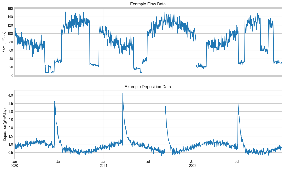
We simulate a bank filtration system with realistic flow patterns and aquifer properties, then create synthetic deposition data to demonstrate the analysis methods.
[2]:
fig, axes = plt.subplots(2, 1, figsize=(14, 8), sharex=True)

# Generate example flow data
date_start = "2020-01-01"
date_end = "2022-12-31"
freq = "D"
example_df, flow_tedges = generate_example_data(date_start=date_start, date_end=date_end, date_freq=freq)
flow_series = example_df["flow"]

# Convert to step format for plotting
axes[0].plot(*step_plot_coords(flow_tedges, flow_series))
axes[0].set_title("Example Flow Data")
axes[0].set_ylabel("Flow (m³/day)")

# Generate example deposition data with seasonal and event patterns
event_dates = pd.to_datetime(["2020-06-15", "2021-03-20", "2021-09-10", "2022-07-05"]).tz_localize("UTC")

deposition_series, deposition_tedges = generate_example_deposition_timeseries(
    date_start=date_start,
    date_end=date_end,
    seasonal_amplitude=0.3,
    noise_scale=0.1,
    event_magnitude=3.0,
    event_duration=30,
    event_decay_scale=10.0,
    event_dates=event_dates,
    ensure_non_negative=True,
)

if not (flow_tedges == deposition_tedges).all():
    msg = "Flow and deposition tedges should align for deposition_to_extraction function"
    raise ValueError(msg)

# Convert to step format for plotting
axes[1].plot(*step_plot_coords(deposition_tedges, deposition_series))
axes[1].set_title("Example Deposition Data")
axes[1].set_ylabel("Deposition (g/m²/day)");
[3]:
# Define aquifer properties for deposition analysis
aquifer_pore_volume = example_df.attrs["aquifer_pore_volume_gamma_mean"]  # m³
retardation_factor = example_df.attrs["retardation_factor"]  # dimensionless

porosity = 0.25  # dimensionless
thickness = 12.0  # m. Aquifer thickness

# Compute derived properties
aquifer_volume = aquifer_pore_volume / porosity  # m³
aquifer_surface_area = aquifer_volume / thickness  # m²
mean_flow = flow_series.mean()  # m³/day
mean_residence_time = aquifer_pore_volume / mean_flow  # days
retarded_residence_time = mean_residence_time * retardation_factor  # days

mean_deposition = deposition_series.mean()  # g/m²/day
mean_extracted_concentration = retarded_residence_time * mean_deposition / (thickness * porosity)  # g/m³

print("Aquifer Properties:")
print(f"Pore volume: {aquifer_pore_volume:.0f} m³")
print(f"Porosity: {porosity:.2f}")
print(f"Thickness: {thickness:.1f} m")
print(f"Surface area: {aquifer_surface_area:.0f} m²")
print(f"Retardation factor: {retardation_factor:.1f}")
print(f"Mean residence time: {mean_residence_time:.1f} days")
print(f"Retarded residence time: {retarded_residence_time:.1f} days")

print("\nApproximate mean concentration in extracted water:")
print(f"Mean deposition: {mean_deposition:.2f} g/m²/day")
print(rf"Mean concentration in extracted water: {mean_extracted_concentration:.2f} g/m³")
Aquifer Properties:
Pore volume: 1000 m³
Porosity: 0.25
Thickness: 12.0 m
Surface area: 333 m²
Retardation factor: 1.0
Mean residence time: 13.3 days
Retarded residence time: 13.3 days

Approximate mean concentration in extracted water:
Mean deposition: 0.91 g/m²/day
Mean concentration in extracted water: 4.00 g/m³
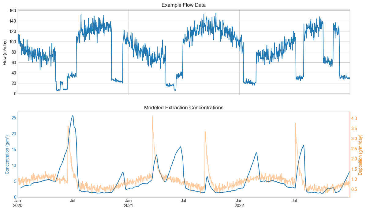
4. Forward Modeling - Predicting Extraction Concentrations#
Using our synthetic deposition data, we predict the concentrations that would be observed in extracted water.
[4]:
print("Computing forward model: deposition → extraction concentrations...")

# Forward modeling: deposition → extraction concentrations
# deposition_to_extraction() requires dep and flow at the same time resolution
modeled_cout = deposition_to_extraction(
    dep=deposition_series,
    flow=flow_series,
    tedges=deposition_tedges,  # time edges for deposition and flow
    cout_tedges=deposition_tedges,
    aquifer_pore_volume=aquifer_pore_volume,
    porosity=porosity,
    thickness=thickness,
    retardation_factor=retardation_factor,
)

# Create concentration series
modeled_cout_series = pd.Series(
    modeled_cout, index=deposition_tedges[1:], name="concentration"
)  # Use the late time edge as index (arbitrary choice)

print("Forward modeling completed")
print(f"Extraction measurements: {len(modeled_cout_series)} samples")
print(f"Concentration range: {modeled_cout_series.min():.1f} - {modeled_cout_series.max():.1f} g/m³")
print(f"Mean concentration: {modeled_cout_series.mean():.1f} g/m³")

# Plot modeled extraction concentrations - convert all series to step format
fig, (ax_flow, ax) = plt.subplots(2, 1, figsize=(14, 8), sharex=True)

# Flow subplot
ax_flow.plot(*step_plot_coords(flow_tedges, flow_series))
ax_flow.set_title("Example Flow Data")
ax_flow.set_ylabel("Flow (m³/day)")

# Concentration subplot
xstep_cout, ystep_cout = step_plot_coords(deposition_tedges, modeled_cout_series)
ax.plot(xstep_cout, ystep_cout, color="C0", alpha=1.0)
ax.set_title("Modeled Extraction Concentrations")
ax.set_ylabel("Concentration (g/m³)", color="C0")
ax.tick_params(axis="y", labelcolor="C0")
ax.spines["left"].set_color("C0")

# Twin axis for deposition
ax2 = ax.twinx()
ax2.plot(*step_plot_coords(deposition_tedges, deposition_series), color="C1", alpha=0.4)
ax2.set_ylabel("Deposition (g/m²/day)", color="C1")
ax2.tick_params(axis="y", labelcolor="C1")
ax2.spines["right"].set_color("C1")

print("Note that the concentration peaks lag behind deposition peaks due to aquifer residence time.")
print("Also, the concentration increases with periods of low flow when residence time is longer.")
print(
    "Also note that for coarser cout_tedges, the mass extracted is conserved and the concentration peaks are smoothed out."
)
Computing forward model: deposition → extraction concentrations...
Forward modeling completed
Extraction measurements: 1096 samples
Concentration range: 1.2 - 18.7 g/m³
Mean concentration: 4.7 g/m³
Note that the concentration peaks lag behind deposition peaks due to aquifer residence time.
Also, the concentration increases with periods of low flow when residence time is longer.
Also note that for coarser cout_tedges, the mass extracted is conserved and the concentration peaks are smoothed out.
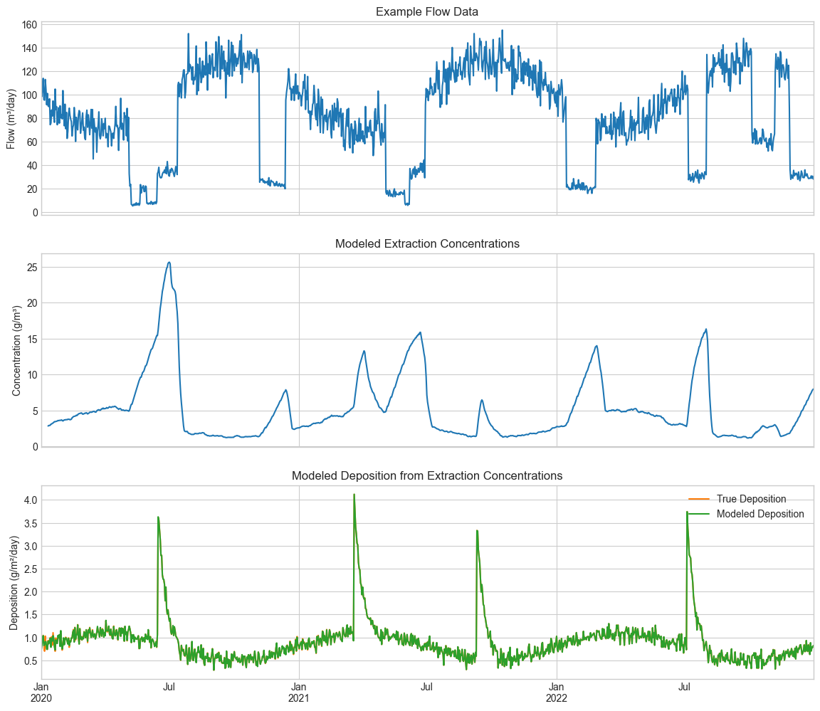
5. Inverse Modeling - Estimating Deposition from Concentrations#
Now we reverse the process: using the calculated concentrations, we estimate the original deposition rates to test our inverse modeling capability.
[5]:
print("Computing inverse model: extraction concentrations → deposition rates...")

# Compute the advective coverage to identify the spin-up period.
# During spin-up, cout is NaN because there is insufficient flow history
# to compute the extraction concentration for the full pore volume.
# fraction_explained_mean returns, per output bin, the advective fraction of the
# bin explained by the flow record (1.0 = fully informed).
frac = rt.fraction_explained_mean(
    flow=flow_series,
    tedges=deposition_tedges,
    cout_tedges=deposition_tedges,
    aquifer_pore_volumes=np.array([aquifer_pore_volume * retardation_factor]),
    direction="extraction_to_infiltration",
)
fully_explained_mask = frac >= 1.0

if fully_explained_mask.any():
    first_fully_explained = example_df.index[fully_explained_mask][0]
    print(f"Spin-up period ends: {first_fully_explained.date()}")
    n_spinup = (~fully_explained_mask).sum()
    print(f"  {n_spinup} days of spin-up excluded from inverse modeling")

# Backward modeling: extraction concentrations → deposition rates
# extraction_to_deposition() requires cout and flow at the same time resolution
# Fill NaN values during spin-up with 0.0 (cout is unknown during spin-up)
modeled_cout_series_fill_nan = modeled_cout_series.fillna(0.0)
modeled_deposition = extraction_to_deposition(
    cout=modeled_cout_series_fill_nan,
    flow=flow_series,
    tedges=deposition_tedges,
    cout_tedges=deposition_tedges,
    aquifer_pore_volume=aquifer_pore_volume,
    porosity=porosity,
    thickness=thickness,
    retardation_factor=retardation_factor,
)
modeled_deposition_series = pd.Series(modeled_deposition, index=deposition_tedges[1:], name="deposition")

print("Basic inverse modeling completed")
print(f"Estimated deposition array shape: {modeled_deposition.shape}")
print(
    f"Deposition range (fully explained): "
    f"{modeled_deposition[fully_explained_mask].min():.2f} - {modeled_deposition[fully_explained_mask].max():.2f} g/m²/day"
)
print(f"Mean deposition (fully explained): {modeled_deposition[fully_explained_mask].mean():.2f} g/m²/day")

# Plot modeled extraction concentrations - convert all series to step format
fig, (ax_flow, ax, ax2) = plt.subplots(3, 1, figsize=(14, 12), sharex=True)

# Flow subplot
ax_flow.plot(*step_plot_coords(flow_tedges, flow_series))
ax_flow.set_title("Example Flow Data")
ax_flow.set_ylabel("Flow (m³/day)")

# Concentration subplot
xstep_cout, ystep_cout = step_plot_coords(deposition_tedges, modeled_cout_series)
ax.plot(xstep_cout, ystep_cout, color="C0", alpha=1.0)
ax.set_title("Modeled Extraction Concentrations")
ax.set_ylabel("Concentration (g/m³)")
ax.grid(True)

# Add fraction explained on twin axis
ax_frac = ax.twinx()
ax_frac.plot(
    *step_plot_coords(deposition_tedges, frac * 100),
    color="gray",
    linewidth=1.5,
    linestyle=":",
    alpha=0.8,
    label="Fraction explained",
)
ax_frac.set_ylabel("Fraction Explained [%]")
ax_frac.set_ylim(0, 105)
ax_frac.legend(loc="lower right", fontsize=9)

# Deposition subplot
xstep_dep_true, ystep_dep_true = step_plot_coords(deposition_tedges, deposition_series)
xstep_dep_model, ystep_dep_model = step_plot_coords(deposition_tedges, modeled_deposition_series)
ax2.plot(xstep_dep_true, ystep_dep_true, color="C1", alpha=1.0, label="True Deposition")
ax2.plot(xstep_dep_model, ystep_dep_model, color="C2", alpha=1.0, label="Modeled Deposition")
ax2.set_title("Modeled Deposition from Extraction Concentrations")
ax2.set_ylabel("Deposition (g/m²/day)")
ax2.grid(True)
ax2.legend(loc="upper right");
Computing inverse model: extraction concentrations → deposition rates...
Spin-up period ends: 2020-01-12
  11 days of spin-up excluded from inverse modeling
Basic inverse modeling completed
Estimated deposition array shape: (1096,)
Deposition range (fully explained): 0.21 - 4.01 g/m²/day
Mean deposition (fully explained): 0.91 g/m²/day
6. Round-Trip Analysis#
Let’s quantify how well our inverse modeling recovered the original deposition pattern by comparing the true and estimated deposition rates.
[6]:
# Quantitative round-trip analysis (fully explained period only)
dep_true = deposition_series.values[fully_explained_mask]
dep_model = modeled_deposition[fully_explained_mask]

correlation = np.corrcoef(dep_true, dep_model)[0, 1]
rmse = np.sqrt(np.mean((dep_true - dep_model) ** 2))
mean_absolute_error = np.mean(np.abs(dep_true - dep_model))
relative_error = np.mean(np.abs(dep_true - dep_model) / dep_true) * 100

print("=== Round-Trip Analysis (fully explained period only) ===")
print("Deposition Recovery Performance:")
print(f"Correlation coefficient: {correlation:.3f}")
print(f"RMSE: {rmse:.3f} g/m²/day")
print(f"Mean absolute error: {mean_absolute_error:.3f} g/m²/day")
print(f"Mean relative error: {relative_error:.1f}%")

# Create comparison scatter plot
fig, (ax1, ax2) = plt.subplots(1, 2, figsize=(15, 6))

# Scatter plot: True vs Estimated (fully explained period only)
ax1.scatter(dep_true, dep_model, alpha=0.6, s=20, color="steelblue")
min_val = min(dep_true.min(), dep_model.min())
max_val = max(dep_true.max(), dep_model.max())
ax1.plot([min_val, max_val], [min_val, max_val], "r--", alpha=0.8, linewidth=2, label="Perfect Match (1:1)")
ax1.set_xlabel("True Deposition [g/m²/day]")
ax1.set_ylabel("Estimated Deposition [g/m²/day]")
ax1.set_title(f"Round-Trip Accuracy (R = {correlation:.3f})")
ax1.legend()
ax1.grid(True, alpha=0.3)

# Time series overlay (first 200 days for clarity) - convert to step format
time_subset = slice(0, 200)
subset_tedges = deposition_tedges[time_subset.start : time_subset.stop + 1]
xstep_subset, ystep_true = step_plot_coords(subset_tedges, deposition_series.values[time_subset])
_, ystep_model = step_plot_coords(subset_tedges, modeled_deposition[time_subset])
ax2.plot(
    xstep_subset,
    ystep_true,
    label="True Deposition",
    color="brown",
    linewidth=2,
    alpha=0.8,
)
ax2.plot(
    xstep_subset,
    ystep_model,
    label="Estimated Deposition",
    color="darkgreen",
    linewidth=2,
    alpha=0.8,
    linestyle="--",
)
ax2.set_xlabel("Date")
ax2.set_ylabel("Deposition [g/m²/day]")
ax2.set_title("Time Series Comparison (First 200 Days)")
ax2.legend()
ax2.grid(True, alpha=0.3)

plt.tight_layout()
plt.show()

print(f"\nKey Insight: The inverse modeling achieves {correlation:.1%} correlation, demonstrating")
print("successful recovery of the original deposition pattern despite the ill-posed nature of the problem.")
=== Round-Trip Analysis (fully explained period only) ===
Deposition Recovery Performance:
Correlation coefficient: 1.000
RMSE: 0.011 g/m²/day
Mean absolute error: 0.008 g/m²/day
Mean relative error: 1.0%
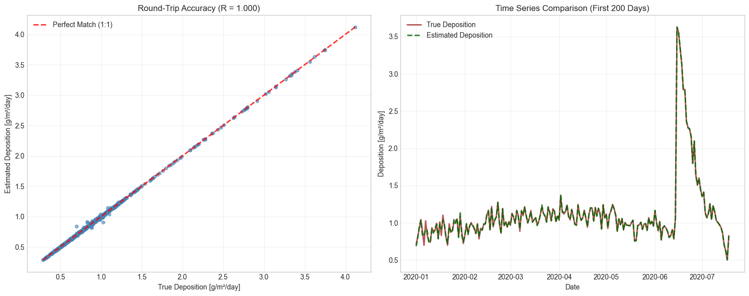
Key Insight: The inverse modeling achieves 100.0% correlation, demonstrating
successful recovery of the original deposition pattern despite the ill-posed nature of the problem.
7. Results & Discussion#
Forward and Inverse Modeling#
Both forward and inverse modeling perform well. The aquifer acts as a low-pass filter, smoothing sharp deposition pulses into broader concentration peaks. Deposition events are clearly visible in concentration responses after residence time delays.
Limitations#
Perfect inverse recovery is limited by aquifer memory effects (temporal smoothing), regularization requirements, and finite data records creating edge effects.
8. Key Takeaways#
Forward and inverse: Complementary tools for prediction and source identification
Temporal dynamics: Residence time distributions control the lag between deposition and extraction
Natural attenuation: Aquifer systems provide beneficial smoothing of concentration peaks
Validation: Synthetic data testing confirms model reliability before field application
9. Engineering Design Considerations#
Model selection: Use forward modeling for scenario analysis, inverse modeling for source identification
Monitoring: Design sampling frequency based on system response time; account for lag times
Risk management: Evaluate scenarios with varying flow rates; plan remediation accounting for delayed response