Note
This notebook is located in the ./examples directory of the gwtransport repository.
Bank filtration with TIMFlow#
gwtransport represents an aquifer as an aquifer pore volume distribution (APVD): a list of pore volumes, one per parallel flow path (“streamtube”), each carrying an equal share of the total flow. From the APVD plus an infiltration time series, gwtransport computes residence times, extraction concentrations / temperatures, and log-removals.
This notebook builds a steady-state analytic-element model of an alternating canal / well-row bank-filtration strip using the TIMFlow PyPI package, traces the equal-flux streamtubes, derives the discrete APVD, and feeds it into gwtransport to produce a realistic multi-year temperature / residence-time / log-removal time series. The TIMFlow model is 2D (vertical cross-section per unit length of well-row into the page), so flow has units of m²/day and pore volumes units of m².
[1]:
# This notebook needs the `timflow` PyPI package in addition to `gwtransport`.
# Install it once with `pip install timflow` (or `uv pip install timflow`).
import sys

try:
    import timflow.steady as tfs
except ImportError:
    print("timflow is not installed; install it with `pip install timflow`.")
    sys.exit(0)

import warnings

import matplotlib.pyplot as plt
import numpy as np
from matplotlib.patches import Polygon, Rectangle

import gwtransport.residence_time as rt
from gwtransport.examples import generate_temperature_example_data
from gwtransport.logremoval import parallel_mean, residence_time_to_log_removal
from gwtransport.utils import step_plot_coords
[2]:
def build_strip_model(
    *,
    width,
    thickness,
    kaq,
    n_por,
    series_of_wells,
    z_well_top,
    z_well_bot,
    h_canal=0.0,
    canal_resistance=1.0,
    canal_width=1.0,
    naq=20,
    kzoverkh=1.0,
):
    """Build a single-aquifer cross-section model of one bank-filtration half-period.

    Covers ``[0, width] x [-thickness, 0]`` with a ``River1D`` canal at
    ``x = 0``, a partially penetrating ``LineSink1D`` well row at
    ``x = width``, and ``ImpermeableWall1D`` symmetry planes at both ends.

    Parameters
    ----------
    width, thickness : float
        Half-period width and aquifer thickness [m].
    kaq : float
        Horizontal hydraulic conductivity [m/day].
    n_por : float
        Effective porosity [-].
    series_of_wells : float
        Total well-row extraction per unit length of row [m²/day].
    z_well_top, z_well_bot : float
        Top and bottom elevation of the well screen [m].
    h_canal : float, optional
        Canal reference head [m].
    canal_resistance : float, optional
        Canal-bed resistance [day].
    canal_width : float, optional
        Canal bed width [m].
    naq : int, optional
        Number of equal vertical sublayers.
    kzoverkh : float, optional
        Vertical-to-horizontal conductivity ratio [-].

    Returns
    -------
    ml : timflow.steady.Model3D
        Solved model.

    Raises
    ------
    ValueError
        If ``z_well_bot`` is not strictly below ``z_well_top``, or if no
        sublayer centre lies within the well screen.
    """
    if z_well_bot >= z_well_top:
        msg = "z_well_bot must be strictly below z_well_top"
        raise ValueError(msg)

    z = np.linspace(0.0, -thickness, naq + 1)
    z_mid = 0.5 * (z[:-1] + z[1:])
    well_layers = np.where((z_mid >= z_well_bot) & (z_mid <= z_well_top))[0]
    if well_layers.size == 0:
        msg = f"No sublayer centre lies within the well screen [{z_well_bot}, {z_well_top}]."
        raise ValueError(msg)
    all_layers = list(range(naq))

    # Tiny inward offset so canal/well do not sit exactly on the symmetry walls.
    offset = 1e-3

    ml = tfs.Model3D(kaq=kaq, z=z, kzoverkh=kzoverkh, npor=n_por, topboundary="conf")
    tfs.River1D(model=ml, xls=offset, hls=h_canal, res=canal_resistance, wh=canal_width, layers=0)
    tfs.LineSink1D(model=ml, xls=width - offset, sigls=series_of_wells / 2.0, layers=well_layers.tolist())
    tfs.ImpermeableWall1D(model=ml, xld=0, layers=all_layers)
    tfs.ImpermeableWall1D(model=ml, xld=width, layers=all_layers)
    ml.solve(silent=True)
    return ml


def locate_streamlines_equal_flux(*, ml, n_start_locs, x_start_loc):
    """Return z-positions on ``x = x_start_loc`` that split flow into equal tubes."""
    qx, _ = ml.disvecalongline(x=[x_start_loc], y=[0.0], layers=None)
    z = np.asarray(ml.aq.find_aquifer_data(x=x_start_loc, y=0.0).z, dtype=float)
    cum = np.pad(np.cumsum(qx[::-1, 0]), (1, 0))
    targets = np.linspace(0.0, cum[-1], n_start_locs + 2)[1:-1]
    return np.interp(targets, cum, z[::-1])


def trace_tubes_bidirectional(*, ml, z_start_locs, x_start_loc, hstepmax=0.5, tmax=1e6, nstepmax=20000, win=None):
    """Trace each start location upstream and downstream and stitch into one pathline."""
    hstepmax = abs(hstepmax)
    z_start_locs = np.asarray(z_start_locs, dtype=float)
    xstart = np.full_like(z_start_locs, x_start_loc)
    ystart = np.zeros_like(z_start_locs)
    common = {"tmax": tmax, "nstepmax": nstepmax, "win": win, "silent": True}
    back_list = tfs.tracelines(ml, xstart, ystart, z_start_locs, -hstepmax, **common)
    fwd_list = tfs.tracelines(ml, xstart, ystart, z_start_locs, hstepmax, **common)

    traces = []
    for back, fwd in zip(back_list, fwd_list, strict=True):
        xyzt_back = back["trace"]
        xyzt_fwd = fwd["trace"]
        tau_back = xyzt_back[-1, 3]
        tau_fwd = xyzt_fwd[-1, 3]

        xyzt_back_rev = xyzt_back[::-1].copy()
        xyzt_back_rev[:, 3] = tau_back - xyzt_back_rev[:, 3]
        xyzt_fwd_shift = xyzt_fwd[1:].copy()
        xyzt_fwd_shift[:, 3] += tau_back

        traces.append({
            "trace": np.vstack([xyzt_back_rev, xyzt_fwd_shift]),
            "message": f"back: {back['message']} | fwd: {fwd['message']}",
            "complete": bool(back["complete"] and fwd["complete"]),
            "tau_back": float(tau_back),
            "tau_fwd": float(tau_fwd),
        })
    return traces


def boundary_edge_trace(*, z_const, x_start, x_end, n_points=100):
    """Return a horizontal streamline trace along a no-flow domain boundary."""
    xs = np.linspace(float(x_start), float(x_end), int(n_points))
    xyzt = np.column_stack([xs, np.zeros_like(xs), np.full_like(xs, float(z_const)), np.zeros_like(xs)])
    return {"trace": xyzt, "message": "no-flow domain boundary", "complete": True}


def trace_streamtube_edges(*, ml, n_tubes, x_start_loc, width, thickness, **trace_kwargs):
    """Return ``n_tubes + 1`` edge traces, ordered from the aquifer floor upwards."""
    defaults = {"hstepmax": 0.5, "tmax": 1e6, "nstepmax": 20000}
    defaults.update(trace_kwargs)
    win = [0.0, width, -0.5, 0.5]
    z_start_locs = locate_streamlines_equal_flux(ml=ml, n_start_locs=n_tubes - 1, x_start_loc=x_start_loc)
    return [
        boundary_edge_trace(z_const=-thickness, x_start=0.0, x_end=width),
        *trace_tubes_bidirectional(ml=ml, z_start_locs=z_start_locs, x_start_loc=x_start_loc, win=win, **defaults),
        boundary_edge_trace(z_const=0.0, x_start=0.0, x_end=width),
    ]


def apvd_from_traces(*, traces_edges, porosity):
    """Return pore volume per streamtube from the shoelace area of edge traces."""
    n_tubes = len(traces_edges) - 1
    pore_vol = np.empty(n_tubes)
    for i in range(n_tubes):
        lower = traces_edges[i]["trace"]
        upper = traces_edges[i + 1]["trace"]
        x = np.concatenate([lower[:, 0], upper[::-1, 0]])
        z = np.concatenate([lower[:, 2], upper[::-1, 2]])
        area = 0.5 * abs(np.sum(x * np.roll(z, -1) - np.roll(x, -1) * z))
        pore_vol[i] = porosity * area
    return pore_vol


def plot_traced_streamlines(*, ax, traces, **kwargs):
    """Draw traced streamlines on ``ax`` and return the line artists."""
    defaults = {"color": "steelblue", "lw": 0.6, "alpha": 0.7}
    defaults.update(kwargs)
    lines = []
    for tr in traces:
        xy = tr["trace"]
        (line,) = ax.plot(xy[:, 0], xy[:, 2], **defaults)
        lines.append(line)
    return lines


def plot_traced_streamtubes(*, ax, traces, shade_colors=("lightgrey", "white"), line_kwargs=None, fontsize=7):
    """Shade streamtubes between consecutive edge traces and number each tube."""
    n_tubes = len(traces) - 1
    artists = []
    for i in range(n_tubes):
        lower = traces[i]["trace"][:, [0, 2]]
        upper = traces[i + 1]["trace"][:, [0, 2]]
        verts = np.vstack([lower, upper[::-1]])
        color = shade_colors[i % len(shade_colors)]
        poly = Polygon(verts, closed=True, facecolor=color, edgecolor="none", zorder=0)
        ax.add_patch(poly)
        artists.append(poly)

    defaults = {"color": "k", "lw": 0.5, "alpha": 0.6}
    if line_kwargs:
        defaults.update(line_kwargs)
    artists.extend(plot_traced_streamlines(ax=ax, traces=traces, **defaults))

    x_min = min(tr["trace"][:, 0].min() for tr in traces)
    x_max = max(tr["trace"][:, 0].max() for tr in traces)
    x_mid = 0.5 * (x_min + x_max)
    dx = 0.01 * (x_max - x_min)
    z_at_mid = [np.interp(x_mid, tr["trace"][:, 0], tr["trace"][:, 2]) for tr in traces]
    for i in range(n_tubes):
        x_lbl = x_mid - dx if i % 2 == 0 else x_mid + dx
        artists.append(
            ax.text(
                x_lbl,
                0.5 * (z_at_mid[i] + z_at_mid[i + 1]),
                str(i),
                ha="center",
                va="center",
                fontsize=fontsize,
                zorder=10,
            )
        )
    return artists


def plot_domain(
    *,
    ax,
    width,
    thickness,
    canal_width=None,
    canal_depth=2.0,
    h_canal=0.0,
    z_well_top=None,
    z_well_bot=None,
    well_x=None,
    well_casing_width=None,
):
    """Draw a conceptual bank-filtration cross-section without grass decoration."""
    artists = []

    rect_x = [0, width, width, 0, 0]
    rect_y = [-thickness, -thickness, 0, 0, -thickness]
    (line,) = ax.plot(rect_x, rect_y, "k-", lw=1.2)
    artists.append(line)

    (m1,) = ax.plot([0, 0], [-thickness, 0], "k--", lw=0.8, alpha=0.5)
    (m2,) = ax.plot([width, width], [-thickness, 0], "k--", lw=0.8, alpha=0.5)
    artists.extend([m1, m2])

    if canal_width is not None:
        canal_half = canal_width / 2.0
        water_top = h_canal
        water_bottom = max(-canal_depth, -thickness)
        water = Rectangle(
            xy=(0.0, water_bottom),
            width=canal_half,
            height=water_top - water_bottom,
            facecolor="#4a90d9",
            edgecolor="#1d4f8a",
            linewidth=1.2,
            alpha=0.55,
            zorder=90,
        )
        ax.add_patch(water)
        artists.append(water)
        (surface,) = ax.plot([0.0, canal_half], [water_top, water_top], color="#1d4f8a", lw=1.5, zorder=91)
        artists.append(surface)

    if z_well_top is not None and z_well_bot is not None:
        xw = float(well_x) if well_x is not None else width
        casing_w = well_casing_width if well_casing_width is not None else 0.02 * width
        casing_top = 0.05 * thickness
        casing = Rectangle(
            xy=(xw - casing_w / 2.0, -thickness),
            width=casing_w,
            height=casing_top - (-thickness),
            facecolor="#b0b0b0",
            edgecolor="black",
            linewidth=1.0,
            zorder=95,
            alpha=0.9,
        )
        ax.add_patch(casing)
        artists.append(casing)

        screen = Rectangle(
            xy=(xw - casing_w / 2.0, z_well_bot),
            width=casing_w,
            height=z_well_top - z_well_bot,
            facecolor="#d94a4a",
            edgecolor="#6b1d1d",
            linewidth=0.8,
            zorder=96,
            alpha=0.4,
        )
        ax.add_patch(screen)
        artists.append(screen)

    ax.set_xlabel("x [m]")
    ax.set_ylabel("z [m]")
    ax.set_xlim(-0.02 * width, 1.02 * width)
    ax.set_ylim(-1.05 * thickness, 0.25 * thickness)
    return artists
[3]:
# Geometry and aquifer properties
width, thickness = 70.0, 25.0  # m
kaq, n_por = 10.0, 0.35  # m/day, -
series_of_wells = 0.01  # m2/day per unit well-row length
z_well_top, z_well_bot = -10.0, -16.0  # m
canal_width, canal_depth = 5.0, 2.0  # m
naq = n_tubes = 25

ml = build_strip_model(
    width=width,
    thickness=thickness,
    kaq=kaq,
    n_por=n_por,
    series_of_wells=series_of_wells,
    z_well_top=z_well_top,
    z_well_bot=z_well_bot,
    canal_width=canal_width,
)
[4]:
# Place tube boundaries at equal-flux intervals on the mid-domain line,
# then trace each one both upstream and downstream.
x_start_loc = width / 2
traces_edges = trace_streamtube_edges(
    ml=ml,
    n_tubes=n_tubes,
    x_start_loc=x_start_loc,
    width=width,
    thickness=thickness,
)
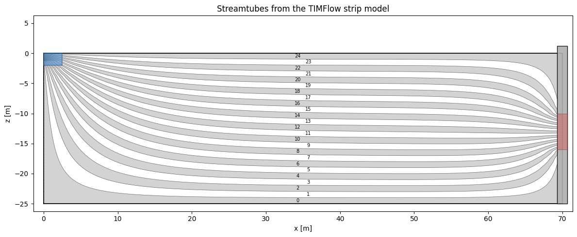
[5]:
# Streamtubes shaded in alternating light grey / white, with tube indices
# matching the bar-chart ordering (tube 0 at the aquifer floor).
fig, ax = plt.subplots(figsize=(12, 5))
plot_traced_streamtubes(ax=ax, traces=traces_edges)
plot_domain(
    ax=ax,
    width=width,
    thickness=thickness,
    canal_width=canal_width,
    canal_depth=canal_depth,
    z_well_top=z_well_top,
    z_well_bot=z_well_bot,
)
ax.set_title("Streamtubes from the TIMFlow strip model")
plt.tight_layout()
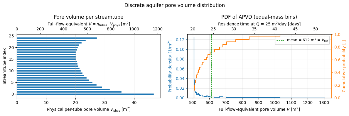
From streamtubes to APVD#
Each streamtube has a physical pore volume \(V_\mathrm{phys} = \text{porosity} \times \text{streamtube area}\). The tubes are placed at equal flux, so every tube carries \(1/n_\mathrm{tubes}\) of the total flow and has probability mass \(1/n_\mathrm{tubes}\) in the distribution.
gwtransport consumes the full-flow-equivalent pore volume \(V = n_\mathrm{tubes} \cdot V_\mathrm{phys}\): the pore volume a homogeneous aquifer would need to reproduce this streamtube’s residence time if it carried the entire flow (\(\tau = V / Q_\mathrm{total}\)). Consequences:
The list of \(V\) values (one per tube) is the APVD that goes into
gwtransport.``mean(apvd) = V_tot`` (total aquifer pore volume); individual \(V_i\) can exceed \(V_\mathrm{tot}\) for slow streamtubes and be below it for fast ones.
This matches what
gwtransport.gamma.bins(...)["expected_values"]returns for a gamma-parameterised APVD.
[6]:
# Discrete APVD as consumed by gwtransport: each equal-flux streamtube is assigned its
# full-flow-equivalent pore volume V_i = tau_i * Q_total = n_tubes * porosity * area_i.
# This matches the convention of `gwtransport.gamma.bins(...)["expected_values"]` (equal
# probability mass 1/n per support point; mean over tubes equals total aquifer pore volume).
apvd = n_tubes * apvd_from_traces(traces_edges=traces_edges, porosity=n_por)

# Mean flow used further below as the residence-time scale on the PDF secondary
# x-axis; also consumed by `generate_temperature_example_data` in the dataset cell.
flow_mean = 25.0  # m^2/day

# Equal-mass bin edges: each equal-flux streamtube is its own bin, with edges at the
# midpoints between sorted support points (outer edges extrapolated symmetrically).
# Every bin carries probability mass 1/n_tubes, matching gwtransport.gamma.bins's
# `probability_mass = 1/n_bins` convention. Bin widths vary, so density =
# (1/n_tubes) / width_i is high where the support is dense and low where it is
# sparse; the integral over all bins is 1 by construction, and the distribution
# mean equals V_tot = total aquifer pore volume.
apvd_sorted = np.sort(apvd)
mids = 0.5 * (apvd_sorted[:-1] + apvd_sorted[1:])
bin_edges = np.concatenate([
    [2 * apvd_sorted[0] - mids[0]],
    mids,
    [2 * apvd_sorted[-1] - mids[-1]],
])

fig, (ax_bar, ax_pdf) = plt.subplots(1, 2, figsize=(12, 4))
fig.suptitle("Discrete aquifer pore volume distribution")

# Left: physical per-tube pore volume. Secondary x-axis shows V = n_tubes * V_phys,
# i.e. the full-flow-equivalent value that is fed into gwtransport as
# `aquifer_pore_volumes`.
ax_bar.barh(range(n_tubes), apvd / n_tubes, height=0.8, edgecolor="white")
ax_bar.set_ylabel("Streamtube index")
ax_bar.set_xlabel(r"Physical per-tube pore volume $V_\mathrm{phys}$ [m$^2$]")
ax_bar.set_title("Pore volume per streamtube")
ax_bar.grid(True, alpha=0.3, axis="x")
secax_bar = ax_bar.secondary_xaxis("top", functions=(lambda v: v * n_tubes, lambda a: a / n_tubes))
secax_bar.set_xlabel(r"Full-flow-equivalent $V = n_\mathrm{tubes} \cdot V_\mathrm{phys}$ [m$^2$]")

# Right: stepped PDF (C0, primary axes) plus empirical CDF on a secondary y-axis
# (C1). Residence time at the mean flow is shown on a secondary x-axis (black).
ax_pdf.hist(apvd, bins=bin_edges, density=True, histtype="step", color="C0", lw=1.5)
ax_pdf.axvline(
    apvd.mean(),
    color="C2",
    ls="--",
    lw=1.0,
    label=rf"mean = {apvd.mean():.0f} m$^2$ = $V_\mathrm{{tot}}$",
)
ax_pdf.set_xlabel(r"Full-flow-equivalent pore volume $V$ [m$^2$]")
ax_pdf.set_ylabel("Probability density [1/m$^2$]", color="C0")
ax_pdf.tick_params(axis="y", colors="C0")
ax_pdf.spines["left"].set_color("C0")
ax_pdf.set_title("PDF of APVD (equal-mass bins)")
ax_pdf.grid(True, alpha=0.3)
ax_pdf.legend(loc="upper right", fontsize=9)

# Secondary y-axis: empirical CDF, stepped at the same bin edges as the PDF so the
# two are visually aligned. Within bin i, F = (i+1)/n_tubes (= cumulative histogram
# mass up to and including that bin).
ax_cdf = ax_pdf.twinx()
ax_cdf.step(
    bin_edges,
    np.linspace(0.0, 1.0, n_tubes + 1),
    where="pre",
    color="C1",
    lw=1.5,
)
ax_cdf.set_ylabel("Cumulative probability [-]", color="C1")
ax_cdf.set_ylim(0, 1)
ax_cdf.tick_params(axis="y", colors="C1")
ax_cdf.spines["right"].set_color("C1")

# Secondary x-axis: residence time at the mean flow, tau = V / flow_mean (default black).
secax_pdf = ax_pdf.secondary_xaxis("top", functions=(lambda v: v / flow_mean, lambda t: t * flow_mean))
secax_pdf.set_xlabel(f"Residence time at Q = {flow_mean:g} m$^2$/day [days]")

plt.tight_layout()
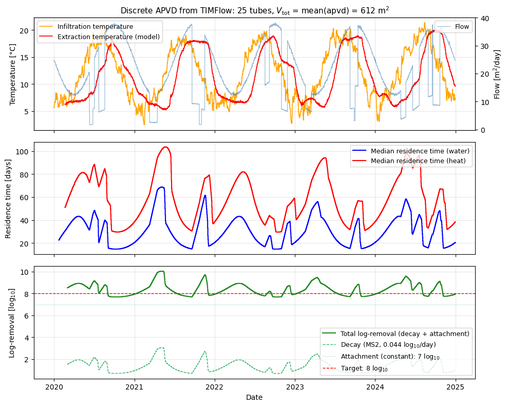
Realistic multi-year dataset#
Feed the streamline-derived discrete APVD into generate_temperature_example_data to obtain a physically consistent dataset: seasonal flow, KNMI-station soil temperature as the infiltration signal, and modelled well-side temperature with thermal retardation (heat travels slower than water because it partitions into the solid matrix) and longitudinal dispersion.
The resulting time series feeds the three-panel figure below:
Temperature + flow — infiltration and modelled extraction temperature.
Median residence time — water vs. heat, the latter longer due to thermal retardation.
Log-removal — two-component pathogen removal model for MS2 (a bacteriophage used as a virus surrogate): temperature-dependent inactivation plus a constant attachment term. Drinking-water guidelines typically target 8 log\(_{10}\) removal for viruses in bank filtration.
[7]:
df, tedges_ts = generate_temperature_example_data(
    date_start="2020-01-01",
    date_end="2024-12-31",
    flow_mean=flow_mean,
    flow_amplitude=12.5,
    flow_noise=0.25,
    cin_method="soil_temperature",
    aquifer_pore_volumes=apvd,
    measurement_noise=0.1,
    streamline_length=width,
)

# Mean residence times per tube over each output interval
rt_water = rt.full(
    flow=df.flow,
    tedges=tedges_ts,
    cout_tedges=tedges_ts,
    aquifer_pore_volumes=apvd,
    retardation_factor=1.0,
    direction="extraction_to_infiltration",
)
rt_thermal = rt.full(
    flow=df.flow,
    tedges=tedges_ts,
    cout_tedges=tedges_ts,
    aquifer_pore_volumes=apvd,
    retardation_factor=df.attrs["retardation_factor"],
    direction="extraction_to_infiltration",
)

# All-NaN slices at the series edges are expected; silence the warning.
with warnings.catch_warnings():
    warnings.filterwarnings("ignore", message="All-NaN slice encountered", category=RuntimeWarning)
    df["rt_water_median"] = np.nanmedian(rt_water, axis=0)
    df["rt_thermal_median"] = np.nanmedian(rt_thermal, axis=0)

# Two-component log-removal: MS2 inactivation at 10 degC plus constant attachment.
log10_decay_rate = np.exp(0.12 * 10 - 3.5) / np.log(10)
lr_attachment = 7.0
log_removal_decay = residence_time_to_log_removal(
    residence_times=rt_water,
    log10_decay_rate=log10_decay_rate,
)
df["lr_decay"] = parallel_mean(log_removals=log_removal_decay, axis=0)
df["lr_total"] = df["lr_decay"] + lr_attachment
[8]:
fig, (ax1, ax2, ax3) = plt.subplots(3, 1, figsize=(10, 8), sharex=True)

# --- Top panel: infiltration / extraction temperature + flow on a twin axis ---
ax1.plot(*step_plot_coords(tedges_ts, df.cin), color="orange", lw=1.2, label="Infiltration temperature")
ax1.plot(*step_plot_coords(tedges_ts, df.cout), color="red", lw=1.2, label="Extraction temperature (model)")
ax1.set_ylabel("Temperature [°C]")
ax1.legend(loc="upper left", fontsize=9)

ax1b = ax1.twinx()
ax1b.plot(*step_plot_coords(tedges_ts, df.flow), color="steelblue", lw=0.8, alpha=0.6, label="Flow")
ax1b.set_ylabel("Flow [m$^2$/day]")
ax1b.legend(loc="upper right", fontsize=9)

ax1.set_title(
    f"Discrete APVD from TIMFlow: {n_tubes} tubes, "
    rf"$V_\mathrm{{tot}}$ = mean(apvd) = {apvd.mean():.0f} m$^2$",
    fontsize=11,
)

# --- Middle panel: median residence time (water and thermal) ---
ax2.plot(
    *step_plot_coords(tedges_ts, df.rt_water_median),
    color="blue",
    lw=1.5,
    label="Median residence time (water)",
)
ax2.plot(
    *step_plot_coords(tedges_ts, df.rt_thermal_median),
    color="red",
    lw=1.5,
    label="Median residence time (heat)",
)
ax2.set_ylabel("Residence time [days]")
ax2.legend(loc="upper right", fontsize=9)

# --- Bottom panel: log-removal (decay + attachment) ---
ax3.plot(
    *step_plot_coords(tedges_ts, df.lr_total),
    color="forestgreen",
    lw=1.5,
    label="Total log-removal (decay + attachment)",
)
ax3.plot(
    *step_plot_coords(tedges_ts, df.lr_decay),
    color="mediumseagreen",
    lw=1.0,
    ls="--",
    label=f"Decay (MS2, {log10_decay_rate:.3f} log$_{{10}}$/day)",
)
ax3.axhline(
    y=lr_attachment,
    color="mediumseagreen",
    ls=":",
    lw=0.8,
    alpha=0.6,
    label=f"Attachment (constant): {lr_attachment:.0f} log$_{{10}}$",
)
ax3.axhline(y=8.0, color="red", ls="--", lw=1.0, label="Target: 8 log$_{10}$")
ax3.set_ylabel("Log-removal [log$_{10}$]")
ax3.set_xlabel("Date")
ax3.legend(loc="lower right", fontsize=9)

for ax in (ax1, ax2, ax3):
    ax.grid(True, alpha=0.3)

plt.tight_layout()