Note

This notebook is located in the ./examples directory of the gwtransport repository.

Advection with Non-Linear Sorption#

This notebook provides a comprehensive guide to solving advection transport with non-linear (Freundlich) sorption using the exact analytical front-tracking method.

Table of Contents#

Theory
- Governing Equation
- Freundlich Sorption Isotherm
- Wave Types
Quick Reference Tables
Examples
- Example 1: Concentration Pulse with Favorable Sorption (n > 1)
- Example 2: Multi-Step Input with Wave Interactions
- Example 3: Concentration Dip with Unfavorable Sorption (n < 1)
Comparison: Effect of Sorption Type on Wave Structure
Notes and Limitations

Theory#

Governing Equation#

The one-dimensional advection equation with sorption in pore volume coordinates \((V, t)\):

\[\frac{\partial C_{\text{total}}}{\partial t} + Q \frac{\partial C}{\partial V} = 0\]

where:

\(C\) is dissolved concentration [mass/volume]
\(C_{\text{total}} = C + \frac{\rho_b}{\theta} s(C)\) is total concentration (dissolved + sorbed per unit pore volume)
\(Q\) is volumetric flow rate [volume/time]
\(V\) is cumulative pore volume [volume]
\(\rho_b\) is bulk density [mass/volume]
\(\theta\) is porosity [-]
\(s(C)\) is sorbed concentration [mass/mass of solid]

This is a hyperbolic conservation law with concentration-dependent wave speeds when sorption is non-linear.

Freundlich Sorption Isotherm#

The Freundlich isotherm relates sorbed and dissolved concentrations:

\[s(C) = k_f C^{1/n}\]

Parameter	Symbol	Units	Description
Freundlich coefficient	\(k_f\)	\((\text{m}^3/\text{kg})^{1/n}\)	Sorption capacity
Freundlich exponent	\(n\)		Isotherm curvature (n=1 is linear)
Bulk density	\(\rho_b\)	kg/m³	Dry mass per bulk volume
Porosity	\(\theta\)		Void fraction

Retardation Factor#

The retardation factor \(R(C)\) relates pore water velocity to concentration velocity:

\[R(C) = 1 + \frac{\rho_b}{\theta} \frac{ds}{dC} = 1 + \frac{\rho_b k_f}{\theta n} C^{(1/n)-1}\]

Key insight: For \(n \neq 1\), \(R\) depends on \(C\), creating concentration-dependent velocities:

\[\lambda(C) = \frac{Q}{R(C)}\]

Regime	Condition	Effect on \(R(C)\)	Physical meaning
Favorable	\(n > 1\)	\(R\) decreases with \(C\)	Higher \(C\) travels faster
Linear	\(n = 1\)	\(R\) constant	All \(C\) travel at same speed
Unfavorable	\(n < 1\)	\(R\) increases with \(C\)	Higher \(C\) travels slower

Wave Types#

Three distinct wave structures arise in hyperbolic conservation laws:

Wave Type	Visualization	Mathematical Form	Physical Process
Characteristic	Single line in V-t space	\(\frac{dV}{dt} = \lambda(C)\)	Smooth regions with constant C
Shock	Sharp front	Rankine-Hugoniot: \(s = \frac{\Delta(QC)}{\Delta C_{\text{total}}}\)	Compression: fast catches slow
Rarefaction	Expanding fan	Self-similar: \(R(C) = \frac{Q(t-t_0)}{V-V_0}\)	Expansion: slow follows fast

Shock Velocity (Rankine-Hugoniot Condition)#

For a discontinuity between \(C_L\) (upstream) and \(C_R\) (downstream):

\[s_{\text{shock}} = \frac{Q(C_R - C_L)}{C_{\text{total}}(C_R) - C_{\text{total}}(C_L)}\]

This ensures mass conservation across the discontinuity.

Entropy Condition (Lax)#

Physical shocks satisfy: \(\lambda(C_L) > s_{\text{shock}} > \lambda(C_R)\)

Characteristics must flow into the shock from both sides.

Quick Reference Tables#

Wave Formation Rules#

	Favorable (\(n > 1\))	Unfavorable (\(n < 1\))
High C velocity	Fast	Slow
Rarefaction when	C decreases	C increases
Shock when	C increases	C decreases

Breakthrough Curve Signatures#

Wave Type	Breakthrough Appearance
Shock	Sharp, instantaneous change
Rarefaction	Gradual, smooth transition
Characteristic	Step change at arrival time

Solver Properties#

Property	Value
Numerical dispersion	Zero
Mass balance precision	Machine precision (~1e-14)
Time stepping	Event-driven (no fixed \(\Delta t\))
Solution type	Exact analytical

[1]:

import matplotlib.pyplot as plt
import numpy as np
import pandas as pd

from gwtransport.advection import infiltration_to_extraction_front_tracking_detailed
from gwtransport.fronttracking.plot import (
    plot_front_tracking_summary,
    plot_sorption_comparison,
)
from gwtransport.fronttracking.validation import verify_physics
from gwtransport.utils import compute_time_edges

plt.rcParams["figure.dpi"] = 100
plt.rcParams["font.size"] = 10

# Common parameters across all examples
bulk_density = 1500.0  # kg/m³
porosity = 0.3

Examples#

Example 1: Concentration Pulse with Favorable Sorption (\(n > 1\))#

A concentration pulse (\(0 \to 10 \to 0\)) demonstrates both shock and rarefaction formation.

Edge	Transition	Wave Type	Reason
Leading	\(0 \to 10\)	Shock	Fast (\(C=10\)) catches slow (\(C=0\))
Trailing	\(10 \to 0\)	Rarefaction	Slow (\(C=0\)) follows fast (\(C=10\))

[2]:

# Example 1: Setup
tedges_ex1 = pd.date_range(start="2020-01-01", periods=100, freq="D")
cin_ex1 = np.zeros(len(tedges_ex1) - 1)
cin_ex1[10:40] = 10.0  # Pulse from day 10 to 40

# Example 1 specific parameters
flow_ex1 = np.full(len(tedges_ex1) - 1, 100.0)  # m³/day
aquifer_pore_volume_ex1 = 200.0  # m³
freundlich_k_ex1 = 0.01  # (m³/kg)^(1/n)
freundlich_n_ex1 = 2.0  # n > 1 (favorable)

cout_tedges_ex1 = pd.date_range(start=tedges_ex1[0], periods=1350, freq="D")

print("Example 1: Concentration Pulse with Favorable Sorption")
print("  Inlet: 0 → 10 (day 10) → 0 (day 40)")
print(f"  Freundlich: n={freundlich_n_ex1}, k={freundlich_k_ex1}")
print(f"  Pore volume: {aquifer_pore_volume_ex1} m³")

Example 1: Concentration Pulse with Favorable Sorption
  Inlet: 0 → 10 (day 10) → 0 (day 40)
  Freundlich: n=2.0, k=0.01
  Pore volume: 200.0 m³

[3]:

# Example 1: Simulation
cout_ex1, structure_ex1 = infiltration_to_extraction_front_tracking_detailed(
    cin=cin_ex1,
    flow=flow_ex1,
    tedges=tedges_ex1,
    cout_tedges=cout_tedges_ex1,
    aquifer_pore_volumes=[aquifer_pore_volume_ex1],
    freundlich_k=freundlich_k_ex1,
    freundlich_n=freundlich_n_ex1,
    bulk_density=bulk_density,
    porosity=porosity,
)

print(
    f"Results: {structure_ex1[0]['n_events']} events | "
    f"{structure_ex1[0]['n_shocks']} shocks | "
    f"{structure_ex1[0]['n_rarefactions']} rarefactions | "
    f"First arrival: {structure_ex1[0]['t_first_arrival']:.1f} days"
)

results_ex1 = verify_physics(structure_ex1[0], cout_ex1, cout_tedges_ex1, cin_ex1, verbose=True)
print(f"\n{results_ex1['summary']}")

Results: 3 events | 1 shocks | 1 rarefactions | First arrival: 27.8 days

✓ All 8 physics checks passed

[4]:

# Example 1: Visualization
axes_ex1 = plot_front_tracking_summary(
    structure_ex1[0],
    tedges_ex1,
    cin_ex1,
    cout_tedges_ex1,
    cout_ex1,
    t_max=150,
    title="Example 1: Pulse with Favorable Sorption (n=2.0)",
)
plt.show()

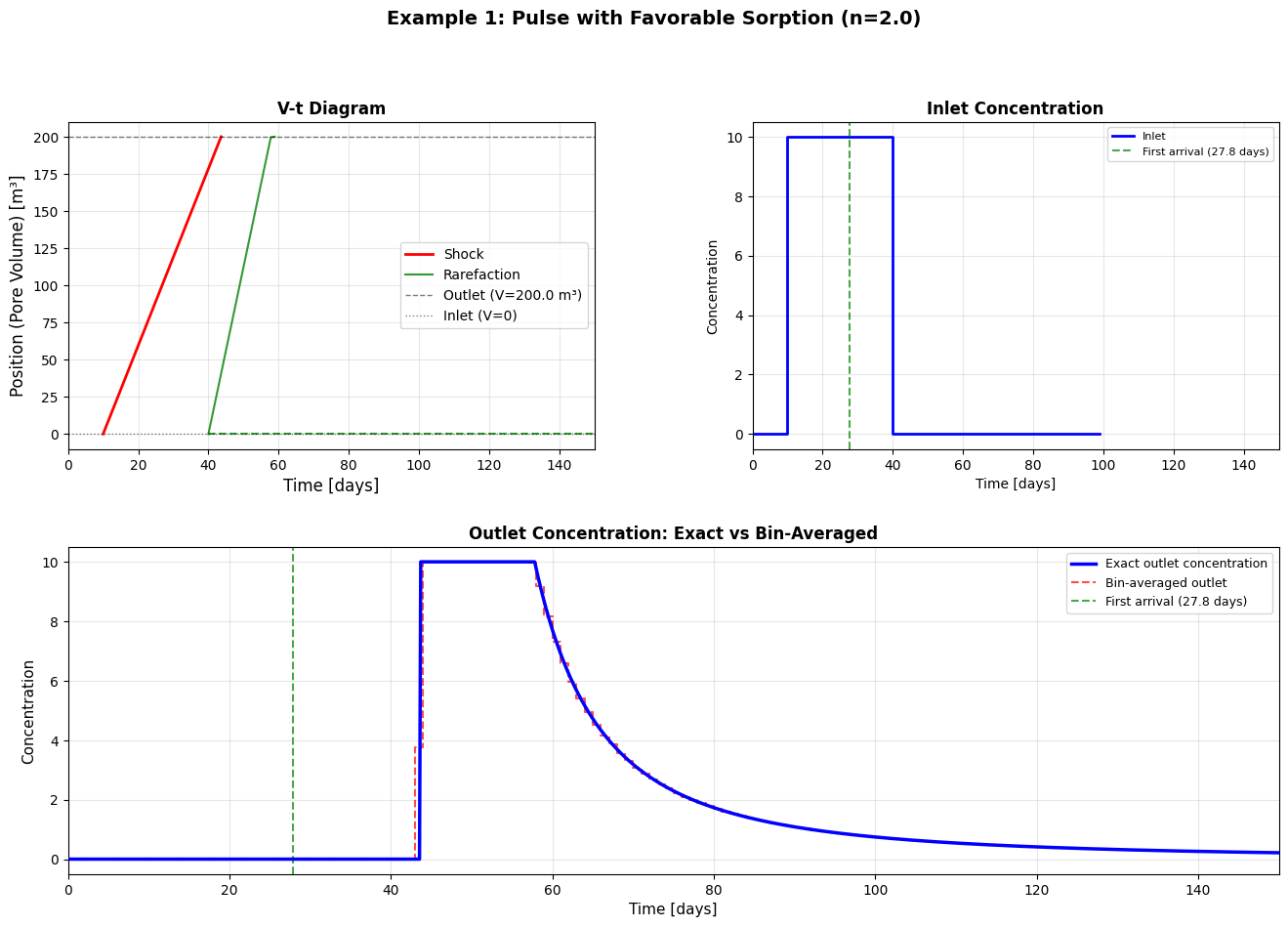
../_images/examples_10_Advection_with_non_linear_sorption_9_0.png

Interpretation: The V-t diagram shows the shock (red) on the leading edge and the rarefaction fan (green) on the trailing edge. The breakthrough curve exhibits a sharp rise followed by a gradual decline.

Example 2: Multi-Step Input with Wave Interactions#

Multiple concentration increases (\(0 \to 10 \to 15 \to 20\)) create interacting shock waves.

Step	Transition	Wave	Interaction Potential
1	\(0 \to 10\)	Shock	Base shock
2	\(10 \to 15\)	Shock	Catches Step 1 (faster)
3	\(15 \to 20\)	Shock	Catches Steps 1-2 (fastest)

[5]:

# Example 2: Setup
tedges_ex2 = pd.date_range(start="2020-01-01", periods=101, freq="D")
cin_ex2 = np.zeros(len(tedges_ex2) - 1)
cin_ex2[10:50] = 10.0  # Step 1
cin_ex2[25:] = 15.0  # Step 2
cin_ex2[30:] = 20.0  # Step 3
cin_ex2[-1] = 0.0  # Return to baseline

# Example 2 specific parameters
flow_ex2 = np.full(len(tedges_ex2) - 1, 100.0)
aquifer_pore_volume_ex2 = 500.0
freundlich_k_ex2 = 0.01
freundlich_n_ex2 = 2.0

cout_tedges_ex2 = pd.date_range(start=tedges_ex2[0], periods=151, freq="D")

print("Example 2: Multi-Step Concentration Increases")
print("  Step 1 (day 10): 0 → 10")
print("  Step 2 (day 25): 10 → 15")
print("  Step 3 (day 30): 15 → 20")
print(f"  Pore volume: {aquifer_pore_volume_ex2} m³")

Example 2: Multi-Step Concentration Increases
  Step 1 (day 10): 0 → 10
  Step 2 (day 25): 10 → 15
  Step 3 (day 30): 15 → 20
  Pore volume: 500.0 m³

[6]:

# Example 2: Simulation
cout_ex2, structure_ex2 = infiltration_to_extraction_front_tracking_detailed(
    cin=cin_ex2,
    flow=flow_ex2,
    tedges=tedges_ex2,
    cout_tedges=cout_tedges_ex2,
    aquifer_pore_volumes=[aquifer_pore_volume_ex2],
    freundlich_k=freundlich_k_ex2,
    freundlich_n=freundlich_n_ex2,
    bulk_density=bulk_density,
    porosity=porosity,
)

print(
    f"Results: {structure_ex2[0]['n_events']} events | "
    f"{structure_ex2[0]['n_shocks']} shocks | "
    f"{structure_ex2[0]['n_rarefactions']} rarefactions | "
    f"First arrival: {structure_ex2[0]['t_first_arrival']:.1f} days"
)

results_ex2 = verify_physics(structure_ex2[0], cout_ex2, cout_tedges_ex2, cin_ex2, verbose=True)
print(f"\n{results_ex2['summary']}")

Results: 7 events | 5 shocks | 1 rarefactions | First arrival: 54.5 days

✓ All 8 physics checks passed

[7]:

# Example 2: Visualization
axes_ex2 = plot_front_tracking_summary(
    structure_ex2[0],
    tedges_ex2,
    cin_ex2,
    cout_tedges_ex2,
    cout_ex2,
    t_max=100,
    show_events=True,
    show_inactive=True,
    title="Example 2: Multi-Step Input with Wave Interactions (n=2.0)",
)
plt.show()

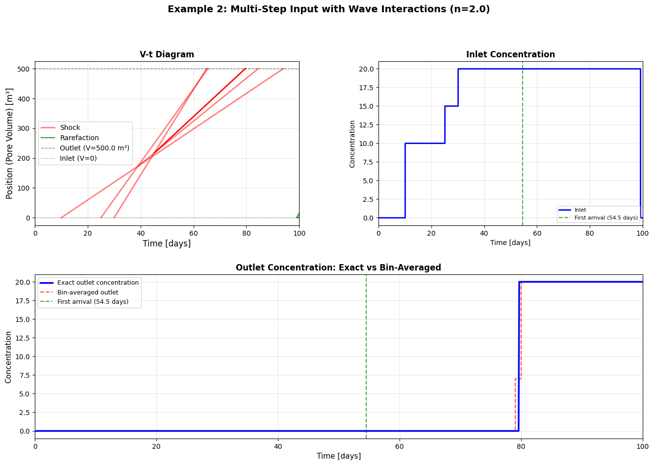
../_images/examples_10_Advection_with_non_linear_sorption_14_0.png

Interpretation: Event markers (×) show where faster shocks catch slower ones. The final breakthrough reaches \(C=20\), the maximum inlet concentration.

Example 3: Concentration Dip with Unfavorable Sorption (\(n < 1\))#

With \(n < 1\), the physics reverses: higher concentrations travel slower.

Property	\(n > 1\) (Favorable)	\(n < 1\) (Unfavorable)
High C velocity	Fast	Slow
Rarefaction from	C decrease	C increase
Shock from	C increase	C decrease

To demonstrate rarefactions with \(n < 1\), we use a concentration dip (\(10 \to 2 \to 10\)):

Edge	Transition	Wave Type	Reason
Leading	\(10 \to 2\)	Rarefaction	Fast (\(C=2\)) outruns slow (\(C=10\))
Trailing	\(2 \to 10\)	Shock	Slow (\(C=10\)) catches fast (\(C=2\))

[8]:

# Example 3: Setup
dates_ex3 = pd.date_range(start="2020-01-01", periods=201, freq="D")
tedges_ex3 = compute_time_edges(tedges=None, tstart=None, tend=dates_ex3, number_of_bins=len(dates_ex3))

cin_ex3 = np.full(len(dates_ex3), 10.0)  # Baseline
cin_ex3[:2] = 0.0  # Initial condition
cin_ex3[40:100] = 2.0  # Dip
cin_ex3[-1] = 0.0  # Explicit end for mass balance

# Example 3 specific parameters
flow_ex3 = np.full(len(dates_ex3), 100.0)
aquifer_pore_volume_ex3 = 200.0
freundlich_k_ex3 = 0.001
freundlich_n_ex3 = 0.7  # n < 1 (unfavorable)

cout_dates_ex3 = pd.date_range(start=dates_ex3[0], periods=300, freq="D")
cout_tedges_ex3 = compute_time_edges(tedges=None, tstart=None, tend=cout_dates_ex3, number_of_bins=len(cout_dates_ex3))

print("Example 3: Concentration Dip with Unfavorable Sorption")
print("  Inlet: 10 → 2 (day 40) → 10 (day 100) → 0 (day 200)")
print(f"  Freundlich: n={freundlich_n_ex3} (n < 1), k={freundlich_k_ex3}")
print("  Physics: High C = High retardation (SLOW)")

Example 3: Concentration Dip with Unfavorable Sorption
  Inlet: 10 → 2 (day 40) → 10 (day 100) → 0 (day 200)
  Freundlich: n=0.7 (n < 1), k=0.001
  Physics: High C = High retardation (SLOW)

[9]:

# Example 3: Simulation
cout_ex3, structure_ex3 = infiltration_to_extraction_front_tracking_detailed(
    cin=cin_ex3,
    flow=flow_ex3,
    tedges=tedges_ex3,
    cout_tedges=cout_tedges_ex3,
    aquifer_pore_volumes=[aquifer_pore_volume_ex3],
    freundlich_k=freundlich_k_ex3,
    freundlich_n=freundlich_n_ex3,
    bulk_density=bulk_density,
    porosity=porosity,
)

print(
    f"Results: {structure_ex3[0]['n_events']} events | "
    f"{structure_ex3[0]['n_shocks']} shocks | "
    f"{structure_ex3[0]['n_rarefactions']} rarefactions | "
    f"First arrival: {structure_ex3[0]['t_first_arrival']:.1f} days"
)

results_ex3 = verify_physics(structure_ex3[0], cout_ex3, cout_tedges_ex3, cin_ex3, verbose=True)
print(f"\n{results_ex3['summary']}")

Results: 8 events | 2 shocks | 2 rarefactions | First arrival: 42.3 days

✓ All 8 physics checks passed

[10]:

# Example 3: Visualization
axes_ex3 = plot_front_tracking_summary(
    structure_ex3[0],
    tedges_ex3,
    cin_ex3,
    cout_tedges_ex3,
    cout_ex3,
    t_max=250,
    title="Example 3: Dip with Unfavorable Sorption (n=0.7)",
)
plt.show()

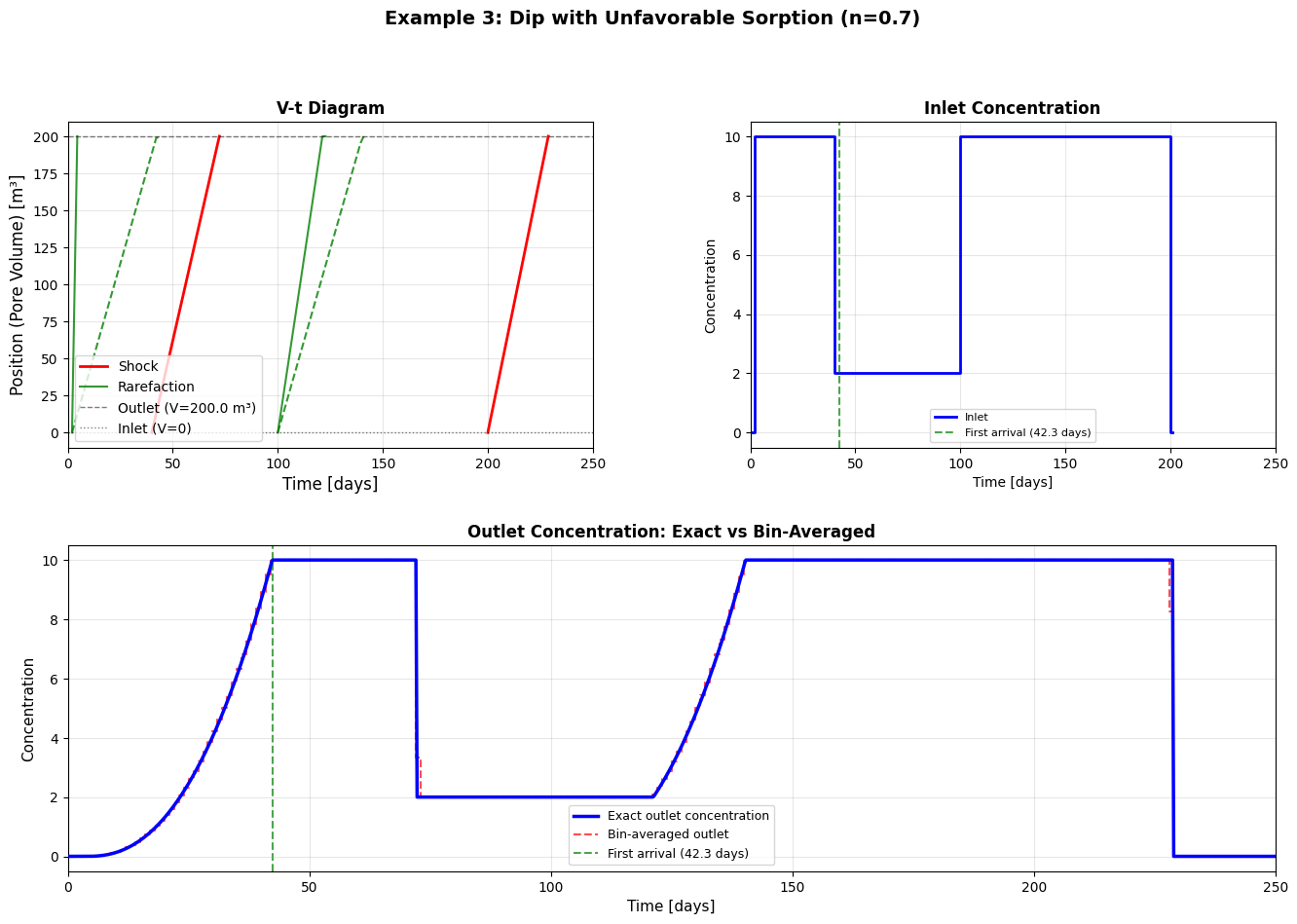
../_images/examples_10_Advection_with_non_linear_sorption_19_0.png

Interpretation: This is the mirror image of Example 1. The rarefaction fan (green) appears on the leading edge (\(10 \to 2\)), while the shock (red) appears on the trailing edge (\(2 \to 10\)).

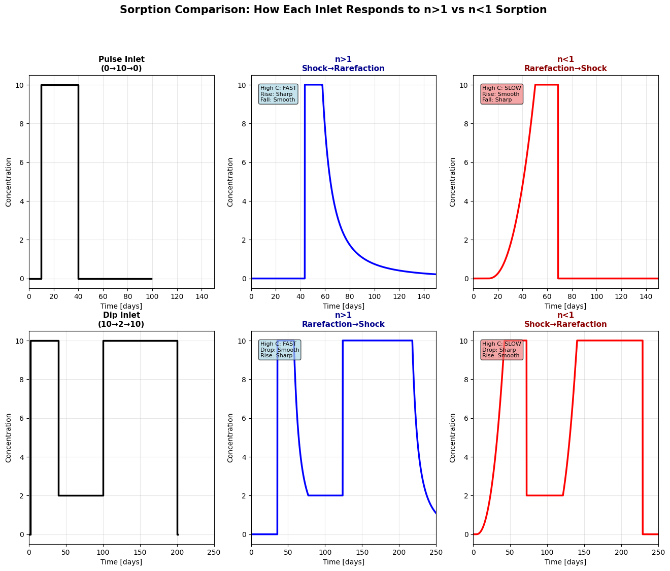
Comparison: Effect of Sorption Type on Wave Structure#

The same inlet pattern produces different wave structures depending on the sorption type.

Inlet	Sorption	Leading Edge	Trailing Edge
Pulse (\(0 \to C \to 0\))	Favorable (\(n>1\))	Shock	Rarefaction
Pulse (\(0 \to C \to 0\))	Unfavorable (\(n<1\))	Rarefaction	Shock
Dip (\(C \to c \to C\))	Favorable (\(n>1\))	Rarefaction	Shock
Dip (\(C \to c \to C\))	Unfavorable (\(n<1\))	Shock	Rarefaction

[11]:

# Cross-comparison: Run pulse with unfavorable and dip with favorable
print("Running pulse inlet with unfavorable sorption (n=0.7)...")
_, structure_pulse_unfav = infiltration_to_extraction_front_tracking_detailed(
    cin=cin_ex1,
    flow=flow_ex1,
    tedges=tedges_ex1,
    cout_tedges=cout_tedges_ex1,
    aquifer_pore_volumes=[aquifer_pore_volume_ex1],
    freundlich_k=freundlich_k_ex3,
    freundlich_n=freundlich_n_ex3,
    bulk_density=bulk_density,
    porosity=porosity,
)

print("Running dip inlet with favorable sorption (n=2.0)...")
_, structure_dip_fav = infiltration_to_extraction_front_tracking_detailed(
    cin=cin_ex3,
    flow=flow_ex3,
    tedges=tedges_ex3,
    cout_tedges=cout_tedges_ex3,
    aquifer_pore_volumes=[aquifer_pore_volume_ex3],
    freundlich_k=freundlich_k_ex1,
    freundlich_n=freundlich_n_ex1,
    bulk_density=bulk_density,
    porosity=porosity,
)

Running pulse inlet with unfavorable sorption (n=0.7)...
Running dip inlet with favorable sorption (n=2.0)...

[12]:

# Comparison plot
fig_comp, axes_comp = plot_sorption_comparison(
    pulse_favorable_structure=structure_ex1[0],
    pulse_unfavorable_structure=structure_pulse_unfav[0],
    pulse_tedges=tedges_ex1,
    pulse_cin=cin_ex1,
    dip_favorable_structure=structure_dip_fav[0],
    dip_unfavorable_structure=structure_ex3[0],
    dip_tedges=tedges_ex3,
    dip_cin=cin_ex3,
    t_max_pulse=150,
    t_max_dip=250,
)
plt.show()

../_images/examples_10_Advection_with_non_linear_sorption_23_0.png

Notes and Limitations#

Only a single compound can be simulated at a time and no chemical reactions are considered. Furthermore, only Freundlich sorption is currently supported, so there is for example no saturation limit. Other isotherms could be implemented without too much effort.

The solver is exact analytical with no numerical dispersion or tolerance-based approximations and is event-driven to track wave interactions precisely. It is mass-conservative to machine precision (~1e-14) and performs physics verification (entropy conditions, arrival times, concentration bounds).

Background Reading#

For the theoretical foundation of non-linear sorption transport, see:

Non-Linear Sorption Concepts - Freundlich isotherm and front-tracking theory
Advection-Dominated Assumption - When diffusion/dispersion is negligible

Implementation Details#

For implementation details, see the API documentation:

gwtransport.fronttracking.math - Sorption models and shock/characteristic velocity
gwtransport.fronttracking.waves - Wave classes (Characteristic, Shock, Rarefaction)
gwtransport.fronttracking.solver - Event-driven simulation engine
infiltration_to_extraction_front_tracking - High-level API