Note

This notebook is located in the ./examples directory of the gwtransport repository.

Open this notebook live in a new tab

Aquifer Storage and Recovery: the buffer effect over repeated cycles

Overview

A single fully-penetrating well injects treated freshwater into a brackish aquifer, the water spreads as a radial bubble, and months later the same well pumps it back – a push–pull / ASR schedule. Mixing at the fresh/brackish interface – microdispersion plus molecular/thermal diffusion – means the recovered water starts fresh and salts up as pumping continues. In practice you stop extracting once the water crosses the potable threshold.

The interesting behaviour is over repeated cycles: freshwater left behind each cycle freshens the aquifer around the well, so the next cycle’s salt-up front arrives later – you recover more usable water before hitting the threshold. This is the buffer effect, the reason real ASR schemes ramp up over their first years. We run three cycles and watch it happen.

gwtransport.radial_asr solves the exact radial advection-dispersion for this push–pull schedule in an infinite aquifer (no grid, no numerical dispersion). We are not running an operational (stop-at-threshold) controller, so we simply preset the signed flow schedule, on irregular time bins – coarse on the flat fresh plateau, finer as the recovered concentration starts to climb and through the threshold, where resolution matters. Every computation includes molecular/thermal diffusion D_m (dominant for heat storage / ATES). Chloride is conservative, so we transport the deviation from the brackish background and add it back.

import matplotlib.pyplot as plt
import numpy as np
import pandas as pd

from gwtransport.radial_asr import infiltration_to_extraction

# --- Site, well, and water chemistry (chloride, mg/L) ---
SCREEN_HEIGHT = 20.0  # m, fully-penetrating well screen
POROSITY = 0.35
WELL_RADIUS = 0.3  # m
ALPHA_L = 0.5  # m, longitudinal dispersivity
MOLECULAR_DIFFUSIVITY = 0.6  # m2/day, molecular/thermal diffusion (heat/ATES scale), included throughout
C_BRACKISH = 1200.0  # native groundwater
C_FRESH = 50.0  # injected treated water
C_POTABLE = 300.0  # usable-water threshold (stop extracting above this)

GEOM = {
    "pore_heights": SCREEN_HEIGHT,
    "porosity": POROSITY,
    "well_radius": WELL_RADIUS,
    "longitudinal_dispersivity": ALPHA_L,
    "molecular_diffusivity": MOLECULAR_DIFFUSIVITY,
}
N_QUAD = 40  # radial resident-profile quadrature (the cost driver when D_m > 0)
INJECTED = 1000.0 * 90  # m3 of freshwater stored per cycle

# Recovery bins, IRREGULAR: coarse on the fresh plateau, finer as cout climbs, fine through the threshold.
RECOVER_DT = [10.0] * 4 + [5.0] * 6 + [2.0] * 15  # 40 + 30 + 30 = 100 days, 25 bins (vs 100 daily)


def schedule(n_cycles):
    """Build (flow rates, bin widths days, time edges, cin) for n_cycles of inject(90 d) + recover(100 d)."""
    segs = ([(1000.0, 90.0)] + [(-800.0, d) for d in RECOVER_DT]) * n_cycles
    flow = np.array([rate for rate, _ in segs])
    dt = np.array([days for _, days in segs])
    tedges = pd.Timestamp("2021-01-01") + pd.to_timedelta(np.concatenate([[0.0], np.cumsum(dt)]), unit="D")
    cin = np.where(flow > 0, C_FRESH, C_BRACKISH)
    return flow, dt, tedges, cin

Three cycles: the salt-up front arrives later each time

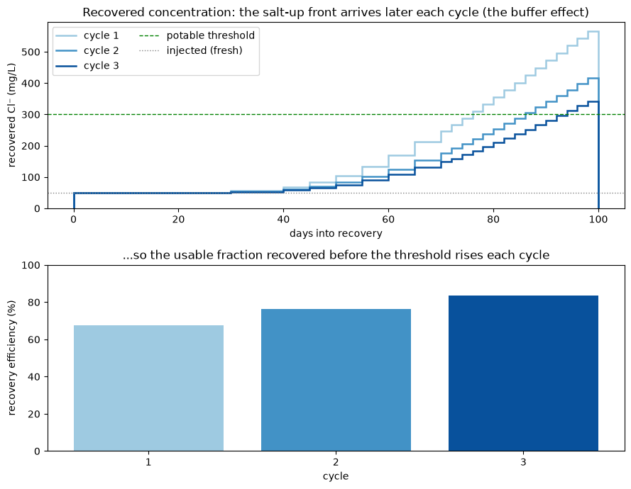
Inject 90,000 m³, recover, repeat – three times. Below we read out the recovered concentration (cout) and, for each cycle, the recovery efficiency: the fraction of the injected volume recovered below the potable threshold (i.e. what you would actually keep if you stopped at the threshold).

n_cycles = 3
flow, dt, tedges, cin = schedule(n_cycles)
cout = infiltration_to_extraction(
    cin=cin,
    flow=flow,
    tedges=tedges,
    cout_tedges=tedges,
    background=C_BRACKISH,
    n_quad=N_QUAD,
    **GEOM,  # ty: ignore[invalid-argument-type]  # the all-float dict widens against `n_modes: int | None`
)

cyc = 1 + len(RECOVER_DT)  # bins per cycle (1 injection + recovery bins)
rec_edges = np.concatenate([[0.0], np.cumsum(RECOVER_DT)])  # recovery-time bin edges (days), same each cycle
vol = np.abs(flow) * dt  # m3 per bin (irregular widths -> volume-weight)

re = []
for k in range(n_cycles):
    sl = slice(k * cyc, (k + 1) * cyc)
    f, v, c = flow[sl], vol[sl], cout[sl]
    e = f < 0
    re.append(np.sum(v[e] * (c[e] < C_POTABLE)) / INJECTED)
    print(f"cycle {k + 1}: recovery efficiency {100 * re[-1]:.0f}%")

fig, (ax0, ax1) = plt.subplots(2, 1, figsize=(9, 7))
colors = ["#9ecae1", "#4292c6", "#08519c"]
for k in range(n_cycles):
    cout_rec = cout[k * cyc + 1 : (k + 1) * cyc]  # the recovery bins of cycle k (injection bin is NaN)
    ax0.stairs(cout_rec, rec_edges, color=colors[k], lw=1.8, label=f"cycle {k + 1}")
ax0.axhline(C_POTABLE, color="green", ls="--", lw=1, label="potable threshold")
ax0.axhline(C_FRESH, color="grey", ls=":", lw=1, label="injected (fresh)")
ax0.set_xlabel("days into recovery")
ax0.set_ylabel("recovered Cl⁻ (mg/L)")
ax0.set_title("Recovered concentration: the salt-up front arrives later each cycle (the buffer effect)")
ax0.legend(ncol=2)

ax1.bar(range(1, n_cycles + 1), [100 * r for r in re], color=colors)
ax1.set_xlabel("cycle")
ax1.set_ylabel("recovery efficiency (%)")
ax1.set_xticks(range(1, n_cycles + 1))
ax1.set_ylim(0, 100)
ax1.set_title("...so the usable fraction recovered before the threshold rises each cycle")
fig.tight_layout()
plt.show()

cycle 1: recovery efficiency 68%
cycle 2: recovery efficiency 76%
cycle 3: recovery efficiency 84%

What the plots show

• Top – the breakthrough moves right. Each cycle the recovered water stays fresh longer and crosses the potable threshold (dashed) later. Operationally you would stop extracting where each curve meets the threshold; we pump a little past only to show the front. The later crossing in cycle 3 is the buffer: the freshwater each previous cycle left behind has freshened the near-well aquifer.

• Bottom – recovery efficiency climbs. The usable fraction recovered before the threshold rises from cycle to cycle, the quantitative signature of the buffer and the reason real ASR yields improve over the first few cycles.

A few modelling notes. The flow is preset (we are not simulating a stop-at-threshold controller), on irregular time bins that are coarse on the flat fresh plateau and fine where cout climbs through the threshold – far fewer steps than daily bins, where it matters. Recovery efficiency is volume-weighted (|flow|·dt) because the bin widths vary, and the breakthrough is drawn as variable-width steps (ax.stairs) – the engine’s output is a flow-weighted bin average. Everything carries molecular/thermal diffusion D_m; cycles are just the sign pattern of flow, composed automatically.

References

• Tang, D. H., & Babu, D. K. (1979). Analytical solution of a velocity dependent dispersion problem. Water Resources Research, 15(6), 1471-1478. — the radial mechanical-dispersion (D = alpha_L |u|) injection solution in Airy functions.

• Aichi, M., & Akitaya, K. (2018). Analytical solution for a radial advection-dispersion equation including both mechanical dispersion and molecular diffusion … from a well. Hydrological Research Letters, 12(3), 23-27. — the D = alpha_L |u| + D_m injection kernel under the same flux boundary.

These treat a single injection; the extraction dual and the multi-cycle push–pull composition shown here are built on top of them.